Migration with surface-related multiples: examples and results
Examples included in the software.
Author: Ning Tu (tning@eos.ubc.ca) Date: Dec/16/2015
Contents
The salt dome examples
In this part, we demonstrate the following points using the salt dome examples:
- Multiples cause artifacts in seismic images if not taken into account.
- Even if we take multiples into account (by including an areal source term in the source wavefield), simply applying the cross-correlation imaging condition is not enough to remove the artifacts.
- We get decent image by inverting the Born scattering operator.
- However, doing inversion is expensive. We reduce the computational cost by subsampling over sources and frequencies, and redraw the subsampling operator for each subproblem (i.e., introducing the message passing term).
- The necessity of redrawing the subsampling operator by comparing with and without redrawing.
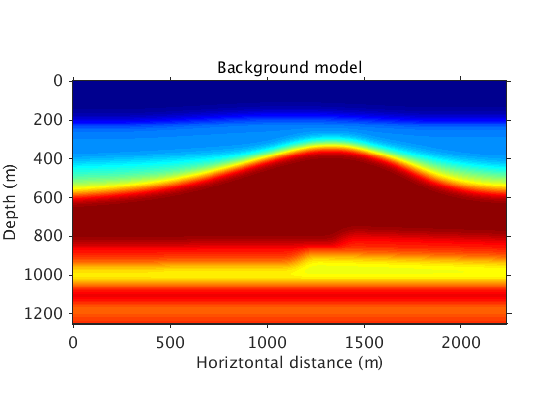
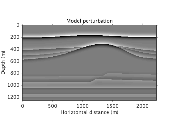
These are the background model and model perturbation:
vel_bg = ['../data/vel_bg_saltdome_mini_slowness2.mat'];
vel_true = ['../data/vel_true_saltdome_mini_slowness2.mat'];
options_file = ['../results/saltdome/precooked/L1Inv_totaldata_2ss15Freq_SourceFreqRenewal_305iter_preview.mat'];
load(vel_bg,'vel_bg')
load(vel_true,'vel_true')
load(options_file,'options')
figure
plot_utils.show_model(vel_bg,options)
title('Background model')
colormap jet
plot_utils.set_my_figure(gca,12)
figure
plot_utils.show_model(1./vel_true.^2-1./vel_bg.^2,options)
title('Model perturbation')
plot_utils.set_my_figure(gca,12)
Showing model...You need to make sure that the model is of correct dimension.
Showing a velocity or density model...
Showing model...You need to make sure that the model is of correct dimension.
Showing a velocity or density model...
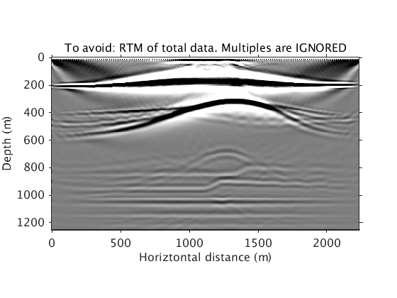
This one shows what you will get if multiples are not correctly handled. In this case, they are simply ignored (pretending there are only primary events, which is not true). We can see the phantom reflectors imaged from them. This shows why you should avoid this scenario and also why conventionally practitioners remove multiples before imaging.
phantom_ref_image = ['../results/saltdome/precooked/RTM_IgnoreMul_FullAcq.mat'];
load(phantom_ref_image,'dm_RTM')
dm_RTM = diff(dm_RTM);
dm_RTM = [dm_RTM(1,:);dm_RTM];
figure
plot_utils.show_model(dm_RTM,options)
caxis([-1 1]*1e10)
title('To avoid: RTM of total data. Multiples are IGNORED')
plot_utils.set_my_figure(gca,12)
Showing model...You need to make sure that the model is of correct dimension.
Showing a velocity or density model...
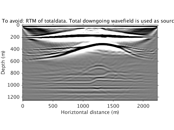
This one shows the non-causal artifacts, by doing cross-correlation migration of the total data by recognizing the total downgoing wavefield as the source. This shows why you should avoid a cross-correlation approach and resort to an inversion approach. Refer to [3] and [4] for more details.
RTM_totaldata_image = ['../results/saltdome/precooked/RTM_totaldata_FullAcq.mat'];
load(RTM_totaldata_image,'dm_RTM')
dm_RTM = diff(dm_RTM);
dm_RTM = [dm_RTM(1,:);dm_RTM];
figure
plot_utils.show_model(dm_RTM,options)
caxis([-1 1]*1e10)
title('To avoid: RTM of totaldata. Total downgoing wavefield is used as source.')
plot_utils.set_my_figure(gca,12)
Showing model...You need to make sure that the model is of correct dimension.
Showing a velocity or density model...
Inversion with sparsity promotion using all sources. The result is clean but the computation is prohibitively expensive.
L1inv_totaldata = ['../results/saltdome/precooked/L1Inv_totaldata_FullAcq_NoRenewal_60iter_preview.mat'];
load(L1inv_totaldata,'dm')
figure
plot_utils.show_model(dm,options)
caxis([-0.2 0.2])
title('L1 migration of total data without subsampling')
plot_utils.set_my_figure(gca,12)
Showing model...You need to make sure that the model is of correct dimension.
Showing a velocity or density model...

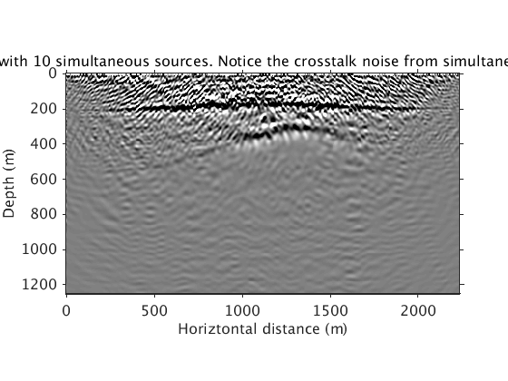
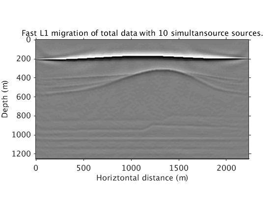
Inversion with sparsity promotion using 10 simultaneous sources and all frequencies. Compared with the above result, a 15X speed up is achieved. Crosstalks from simultaneous sources, shown in the RTM image, are suppressed in the inverted image.
Totaldata_smallbatch = ['../results/saltdome/precooked/L1Inv_totaldata_2ss15Freq_SourceFreqRenewal_305iter_preview.mat'];
load(Totaldata_smallbatch,'dm_RTM')
dm_RTM = diff(dm_RTM);
dm_RTM = [dm_RTM(1,:);dm_RTM];
figure
plot_utils.show_model(dm_RTM,options)
plot_utils.set_my_figure(gca,12)
caxis([-1 1]*1e10)
title('Migration with 10 simultaneous sources. Notice the crosstalk noise from simultaneous sources.')
load(Totaldata_smallbatch,'dm')
figure
plot_utils.show_model(dm,options)
plot_utils.set_my_figure(gca,12)
caxis([-0.2 0.2])
title('Fast L1 migration of total data with 10 simultansource sources.')
Showing model...You need to make sure that the model is of correct dimension.
Showing a velocity or density model...
Showing model...You need to make sure that the model is of correct dimension.
Showing a velocity or density model...
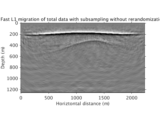
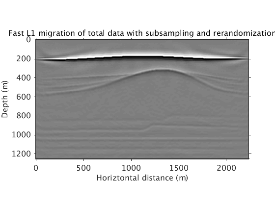
Inversion with sparsity promotion using 2 simultaneous sources, 15 frequencies, and 305 iterations. This combination leads to a number of PDE solves that is the same as a single reverse time migration with full data. However, this subsampling ratio leads to significant artifacts in the image. We propose to remove these artifacts by drawing new subsets of sources and freqs for each subproblem.
L1inv_totaldata_minibatch_norenew = ['../results/saltdome/precooked/L1Inv_totaldata_2ss15Freq_NoRenewal_305iter_preview.mat'];
load(L1inv_totaldata_minibatch_norenew,'dm')
figure
plot_utils.show_model(dm,options)
plot_utils.set_my_figure(gca,12)
caxis([-0.2 0.2])
title('Fast L1 migration of total data with subsampling without rerandomization')

L1inv_totaldata_minibatch = ['../results/saltdome/precooked/L1Inv_totaldata_2ss15Freq_SourceFreqRenewal_305iter_preview.mat'];
load(L1inv_totaldata_minibatch,'dm')
figure
plot_utils.show_model(dm,options)
plot_utils.set_my_figure(gca,12)
caxis([-0.2 0.2])
title('Fast L1 migration of total data with subsampling and rerandomization')
Showing model...You need to make sure that the model is of correct dimension.
Showing a velocity or density model...
Showing model...You need to make sure that the model is of correct dimension.
Showing a velocity or density model...
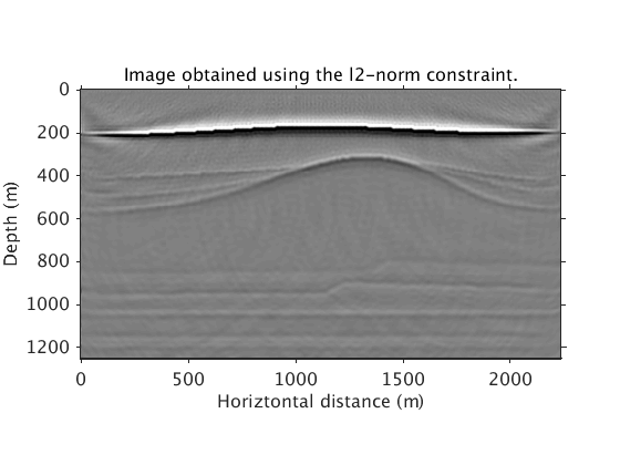
We show that the l1 sparsity constraint is necessary, by comparing with the image obtained using l2 constraint
L2Pinv_totaldata_minibatch = ['../results/saltdome/precooked/L2PInv_totaldata_2ss15Freq_SourceFreqRenewal_305iter_preview.mat'];
load(L2Pinv_totaldata_minibatch,'dm')
figure
plot_utils.show_model(dm,options)
plot_utils.set_my_figure(gca,12)
caxis([-0.2 0.2])
title('Image obtained using the l2-norm constraint.')
Showing model...You need to make sure that the model is of correct dimension.
Showing a velocity or density model...
Examples using the sedimentary part of the Sigsbee 2B model
data modelling using iWave w/ free-surface boundary condition data inversion using our in-house frequency-domain modelling
options.color_model = 'gray';
options.dx = 7.62;
options.dz = 7.62;
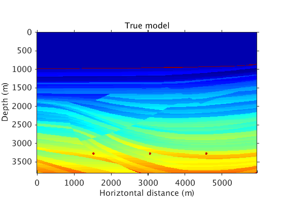
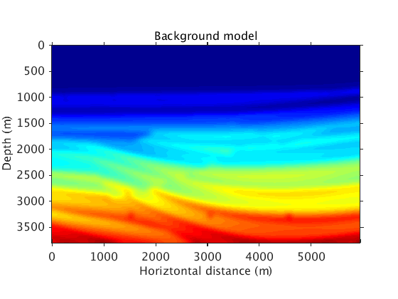
The true and background models.
vel = ['../data/sigsbee_nosalt_model.mat'];
load(vel,'vel_bg')
load(vel,'vel_true')
figure
plot_utils.show_model(vel_true,options)
title('True model')
colormap jet
plot_utils.set_my_figure(gca,12)
figure
plot_utils.show_model(vel_bg,options)
title('Background model')
colormap jet
plot_utils.set_my_figure(gca,12)
Showing model...You need to make sure that the model is of correct dimension.
Showing a velocity or density model...
Showing model...You need to make sure that the model is of correct dimension.
Showing a velocity or density model...
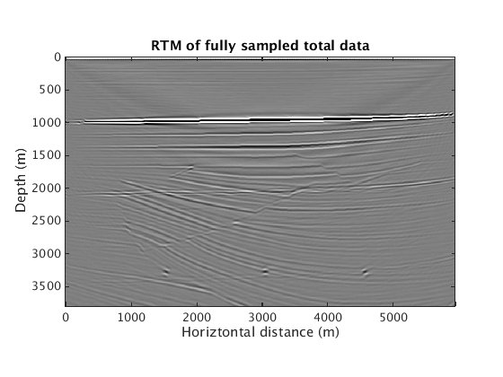
Again RTM with multiples leads to spurious artifacts
RTM_totaldata_SGB = ['../results/sigsbee/precooked/RTMTotalFD_iwave_TrueQ.mat'];
load(RTM_totaldata_SGB,'dm_RTM')
figure
plot_utils.show_model(dm_RTM,options)
caxis([-1 1]*1e4)
title('RTM of fully sampled total data')
Showing model...You need to make sure that the model is of correct dimension.
Showing a velocity or density model...
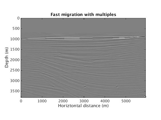
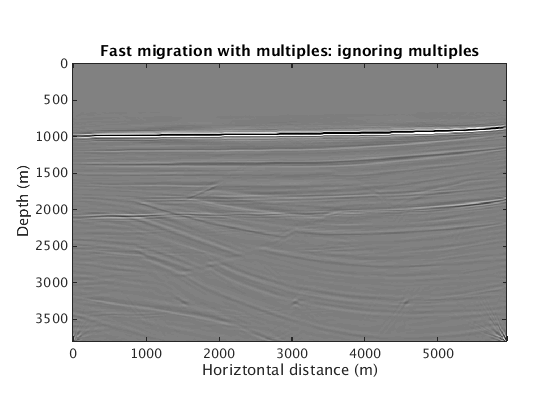
Inversion with multiples leads to a clean image. Computational cost again roughly rivals one RTM w/ all the data. Ignoring the presence of multiples leads again to spurious artifacts.
L1inv_totaldata_SGB = ['../results/sigsbee/precooked/MigTotalFD_iwave_26ss31freq_bg_TrueQ_GaussianEnc_denoised.mat'];
load(L1inv_totaldata_SGB,'dm')
figure
plot_utils.show_model(dm,options)
caxis([-0.1 0.1])
title('Fast migration with multiples')

L1inv_totaldata_IgnMul_SGB = ['../results/sigsbee/precooked/MigTotalFD_iwave_26ss31freq_bg_TrueQ_GaussianEnc_IgnoreMul_denoised.mat'];
load(L1inv_totaldata_IgnMul_SGB,'dm')
figure
plot_utils.show_model(dm,options)
caxis([-0.1 0.1])
title('Fast migration with multiples: ignoring multiples')
Showing model...You need to make sure that the model is of correct dimension.
Showing a velocity or density model...
Showing model...You need to make sure that the model is of correct dimension.
Showing a velocity or density model...
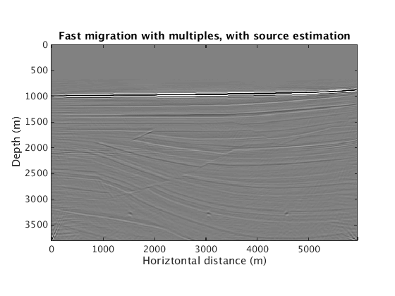
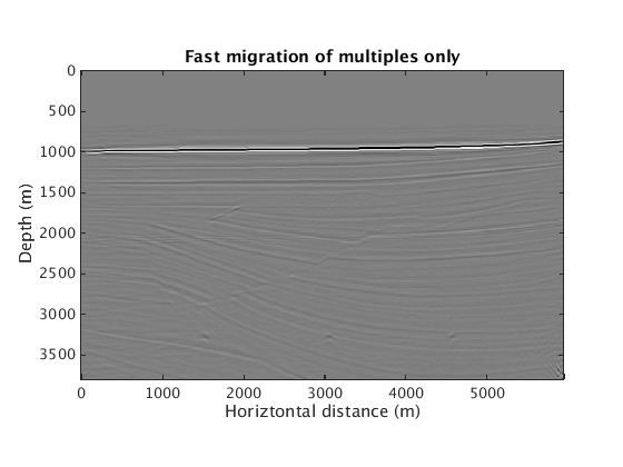
When exact knowledge of the source wavelet is not known, we can either estimate the source wavelet or, if a good primary/multiple separation can be achieved, image multiple-only data.
L1inv_totaldata_EQ_SGB = ['../results/sigsbee/precooked/MigTotalFD_iwave_26ss31freq_EstQ_GausEnc_denoised.mat'];
load(L1inv_totaldata_EQ_SGB,'dm')
figure
plot_utils.show_model(dm,options)
caxis([-0.1 0.1]*0.025)
title('Fast migration with multiples, with source estimation')

L1inv_mul_SGB = ['../results/sigsbee/precooked/MigTotalFD_Mul_iwave_26ss31freq_bg_GaussianEncoding_denoised.mat'];
load(L1inv_mul_SGB,'dm')
figure
plot_utils.show_model(dm,options)
caxis([-0.1 0.1])
title('Fast migration of multiples only')
Showing model...You need to make sure that the model is of correct dimension.
Showing a velocity or density model...
Showing model...You need to make sure that the model is of correct dimension.
Showing a velocity or density model...
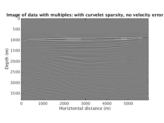
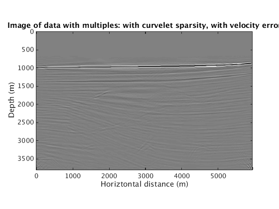
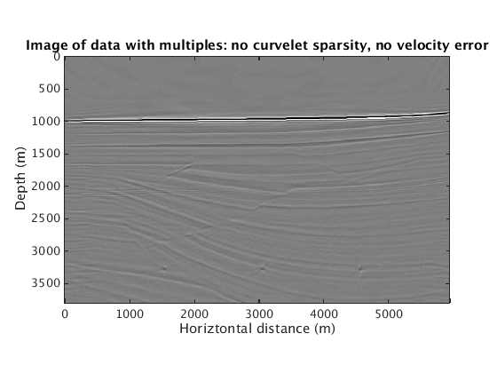
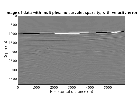
When the velocity model is wrong, how does the proposed method behave? We find that sparsity promotion in the curvelet domain improves the robustness of the method to velocity errors. The following results show the comparison with and without curvelet-domain sparsity promotion, with and without the velocity errors.
L1inv_totaldata_SGB = ['../results/sigsbee/precooked/MigTotalFD_iwave_26ss31freq_bg_TrueQ_GaussianEnc_denoised.mat'];
load(L1inv_totaldata_SGB,'dm')
figure
plot_utils.show_model(dm,options)
caxis([-0.1 0.1])
title('Image of data with multiples: with curvelet sparsity, no velocity error')

L1inv_totaldata_KWM_SGB = ['../results/sigsbee/precooked/KWModelUnder2X_MigTotalFD_iwave_26ss31freq_bg_TrueQ_GaussianEnc_denoised.mat'];
load(L1inv_totaldata_KWM_SGB,'dm')
figure
plot_utils.show_model(dm,options)
caxis([-0.1 0.1])
title('Image of data with multiples: with curvelet sparsity, with velocity error')

RBK_totaldata_SGB = ['../results/sigsbee/precooked/MigTotalFD_iwave_26ss31freq_bg_TrueQ_GaussianEnc_RBK_NoCurv_denoised.mat'];
load(RBK_totaldata_SGB,'dm')
figure
plot_utils.show_model(dm,options)
caxis([-0.1 0.1])
title('Image of data with multiples: no curvelet sparsity, no velocity error')

RBK_totaldata_KWM_SGB = ['../results/sigsbee/precooked/KWModelUnder2X_MigTotalFD_iwave_26ss31freq_bg_TrueQ_GaussianEnc_RBK_NoCurv_denoised.mat'];
load(RBK_totaldata_KWM_SGB,'dm')
figure
plot_utils.show_model(dm,options)
caxis([-0.1 0.1])
title('Image of data with multiples: no curvelet sparsity, with velocity error')
Showing model...You need to make sure that the model is of correct dimension.
Showing a velocity or density model...
Showing model...You need to make sure that the model is of correct dimension.
Showing a velocity or density model...
Showing model...You need to make sure that the model is of correct dimension.
Model data contain complex numbers. Only real part is shown
Showing a velocity or density model...
Showing model...You need to make sure that the model is of correct dimension.
Model data contain complex numbers. Only real part is shown
Showing a velocity or density model...