2D Efficient least-squares imaging with sparsity promotion and compressive sensing

       Seismic Laboratory for Imaging and Modeling
       Department of Earch & Ocean Sciences
       The University of British Columbia

Contents

One-layer example

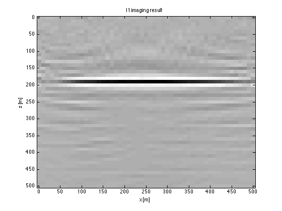
This is an demonstration of l1 migration algorithm based on One-layer model, please visit the script 'MGNFWI_camenbert.m' for detail

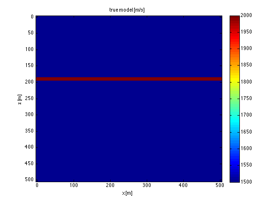
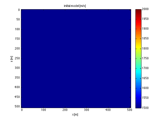
true model and initial model

z = 0:10:500;
x = 0:10:500;
vel = 1500*ones(51,51);
vel(20,:)=2000;
vels = 1500*ones(51,51);

%
figure(1);imagesc(x,z,vel);caxis([1500,2000]);xlabel('x [m]');ylabel('z [m]');title('true model [m/s]');colorbar;
figure(2);imagesc(x,z,vels);caxis([1500,2000]);xlabel('x [m]');ylabel('z [m]');title('initial model [m/s]');colorbar;

% l1 migration

% reflection example, source and receivers are on the top of the model

load LSM_Toy_model_L1_WRSeqOffset3Shots3FsIvc.mat
figure(3);imagesc(x,z,updates(:,:,13));colormap gray;xlabel('x [m]');ylabel('z [m]');title('l1 imaging result');

BG model example

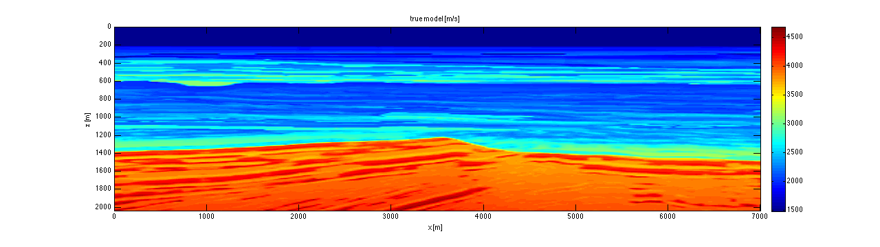
This is an demonstration of l1 migration algorithm based on BG Compass model [1,2], please visit the script MGNFWI_BG.html for detail

true model and initial model

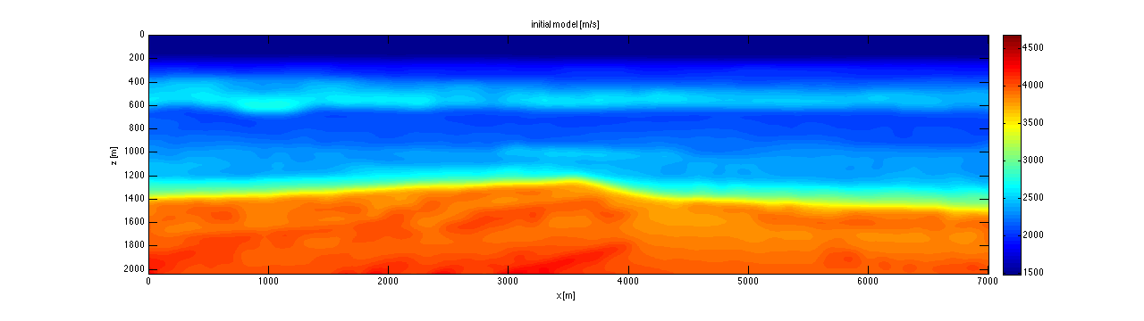
load BG_compass_model409x1401.mat
z = 0:5:2040;
x = 0:5:7000;
scrsz = get(0,'ScreenSize');
figure('Position',[1 scrsz(4)/4 scrsz(3)/2 scrsz(4)/4]);imagesc(x,z,vel);set(gca,'plotboxaspectratio',[7 2 2]);caxis([1480,4680]);xlabel('x [m]');ylabel('z [m]');title('true model [m/s]');colorbar;

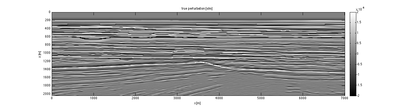
scrsz = get(0,'ScreenSize');
figure('Position',[1 scrsz(4)/4 scrsz(3)/2 scrsz(4)/4]);imagesc(x,z,vels);set(gca,'plotboxaspectratio',[7 2 2]);caxis([1480,4680]);xlabel('x [m]');ylabel('z [m]');title('initial model [m/s]');colorbar;

scrsz = get(0,'ScreenSize');
figure('Position',[1 scrsz(4)/4 scrsz(3)/2 scrsz(4)/4]);imagesc(x,z,diff(1./vels-1./vel));set(gca,'plotboxaspectratio',[7 2 2]);caxis(1e-5*[-2 2]);xlabel('x [m]');ylabel('z [m]');title('true perturbation [s/m]');colorbar;colormap gray

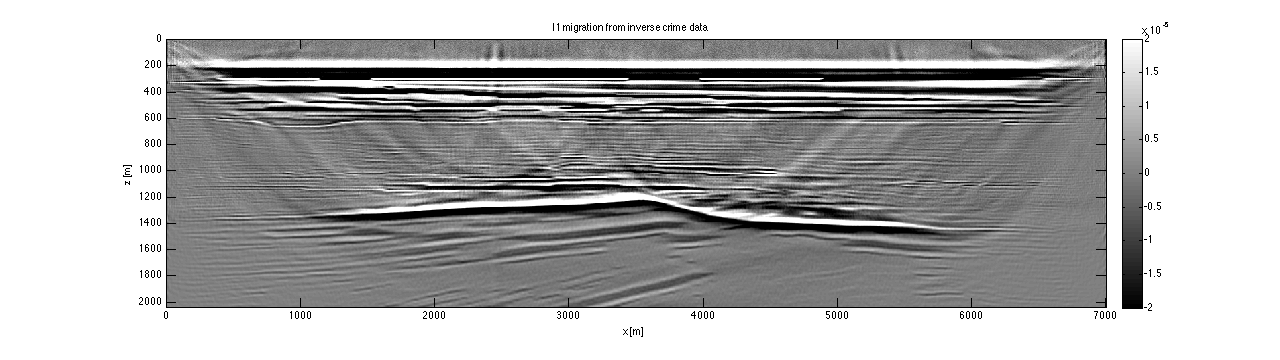
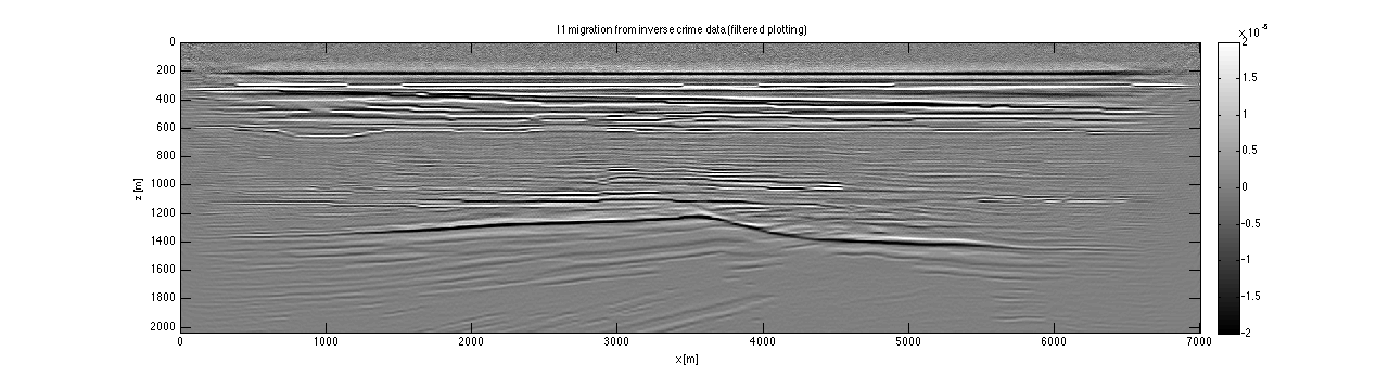
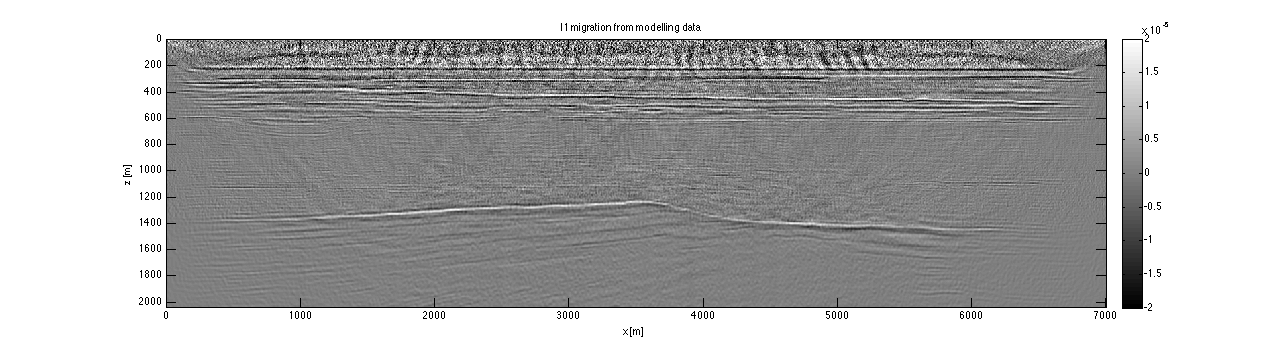
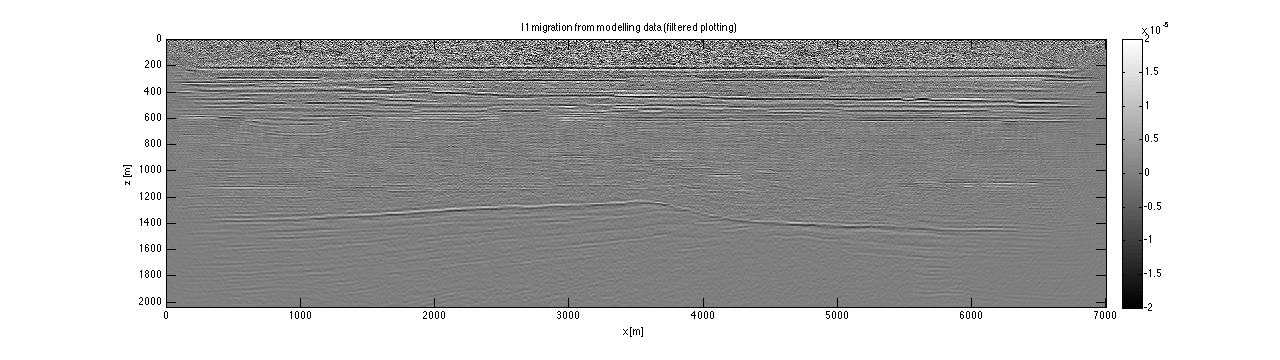
% L1 migration with 3 simultaneous shots and 10 frequencies
% in this case we use inverse crime data to test our algorithm

load LSM_BGcompass_model2d_L1_WRSim3Shots10FsIvc.mat

scrsz = get(0,'ScreenSize');
figure('Position',[1 scrsz(4)/4 scrsz(3)/2 scrsz(4)/4]);imagesc(x,z,updates(:,:,end));set(gca,'plotboxaspectratio',[7 2 2]);caxis(1e-5*[-2 2]);xlabel('x [m]');ylabel('z [m]');title('l1 migration from inverse crime data');colorbar;colormap gray


% plot differential of the image to get rid of those low frequency turning wave compenents
scrsz = get(0,'ScreenSize');
figure('Position',[1 scrsz(4)/4 scrsz(3)/2 scrsz(4)/4]);imagesc(x,z,diff(updates(:,:,end)));set(gca,'plotboxaspectratio',[7 2 2]);caxis(1e-5*[-2 2]);xlabel('x [m]');ylabel('z [m]');title('l1 migration from inverse crime data (filtered plotting)');colorbar;colormap gray



% L1 migration with 3 simultaneous shots and 10 frequencies
% in this case we use wavefield from frequency domain forward modeling method to test our algorithm
load LSM_BGcompass_model2d_L1_WRSim3Shots10Fs.mat

scrsz = get(0,'ScreenSize');
figure('Position',[1 scrsz(4)/4 scrsz(3)/2 scrsz(4)/4]);imagesc(x,z,updates(:,:,end));set(gca,'plotboxaspectratio',[7 2 2]);caxis(1e-5*[-2 2]);xlabel('x [m]');ylabel('z [m]');title('l1 migration from modelling data');colorbar;colormap gray


% plot differential of the image to get rid of those low frequency turning wave compenents
scrsz = get(0,'ScreenSize');
figure('Position',[1 scrsz(4)/4 scrsz(3)/2 scrsz(4)/4]);imagesc(x,z,diff(updates(:,:,end)));set(gca,'plotboxaspectratio',[7 2 2]);caxis(1e-5*[-2 2]);xlabel('x [m]');ylabel('z [m]');title('l1 migration from modelling data (filtered plotting)');colorbar;colormap gray