![]()
![]()
Abstract
Devito is an open-source Python project based on domain-specific language and compiler technology. Driven by the requirements of rapid HPC applications development in exploration seismology, the language and compiler have evolved significantly since inception. Sophisticated boundary conditions, tensor contractions, sparse operations and features such as staggered grids and sub-domains are all supported; operators of essentially arbitrary complexity can be generated. To accommodate this flexibility whilst ensuring performance, data dependency analysis is utilized to schedule loops and detect computational-properties such as parallelism. In this article, the generation and simulation of MPI-parallel propagators (along with their adjoints) for the pseudo-acoustic wave-equation in tilted transverse isotropic media and the elastic wave-equation are presented. Simulations are carried out on industry scale synthetic models in a HPC Cloud system and reach a performance of 28TFLOP/s, hence demonstrating Devito’s suitability for production-grade seismic inversion problems.
Introduction
Seismic imaging methods such Reverse Time Migration (RTM) and Full-waveform inversion (FWI) rely on the numerical solution of an underlying system of partial differential equations (PDEs), most commonly some manifestation of the wave-equation. In the context of FWI, the finite-difference (FDM) and the spectral-element (SEM) methods are most frequently used to solve the wave-equation, with FDM methods dominating within the seismic exploration community (Lyu et al., 2020). Various forms of the wave-equation and modelling strategies for FWI are detailed in (Fichtner, 2010).
Despite the theory of FWI dating back to the 1980s (Tarantola, 1984), among the first successful expositions on real 3D data was presented in (Sirgue et al., 2009). Other studies utilizing FDM within the FWI workflow include (Ratcliffe et al., 2011; Petersson and Sjögreen, 2014). The aforementioned studies approximate the underlying physics via the acoustic wave-equation; higher fidelity models solving the non-isotropic elastic wave-equation have been developed in, e.g., (Preston, 2018, 2019a, 2019b; Köhn et al., 2015; Zehner et al., 2016). Owing to the flexibility of the mathematical discretizations that can be utilized, along with the ability to describe problems on complex meshes, there has also been a great deal of interest in utilizing SEM to solve inversion problems (Peter et al., 2011; Krebs et al., 2014). The recent study (Trinh et al., 2019) presents an efficient SEM based inversion scheme using a viscoelastic formulation of the wave-equation.
It is generally accepted that the PDE solver utilized within an inversion workflow must satisfy the following criteria (Virieux et al., 2009): - Efficient for multiple-source modelling - The memory requirement of the modelling - The ability of a parallel algorithm to use an increasing number of processors - Ability of the method to process models of arbitrary levels of heterogeneity - Reduce the nonlinearity of FWI - Feasibility of the extension of the modelling approach to more realistic physical descriptions of the media.
It is with these specifications in mind that Devito, a symbolic domain specific language (DSL) and compiler for the automatic generation of finite-difference stencils, has been developed. Originally deigned to accelerate research and development in exploration geophysics, the high-level interface, previously described in detail in (M. Louboutin et al., 2019), is built on top of SymPy (Meurer et al., 2017) and is inspired by the underlying mathematical formulations and other DSLs such as FEniCS (Logg et al., 2012) and Firedrake (Rathgeber et al., 2015). This interface allows the user to formulate wave-equations, and more generally time-dependent PDEs in a simple and mathematically coherent way. The Devito compiler then automatically generates finite-difference stencils from these mathematical expressions. One of the main advantages of Devito over other finite-difference DSLs is that generic expressions such as sparse operations (i.e. point source injection or localized measurements) are fully supported and expressible in a high-level fashion. The second component of Devito is its compiler (c.f (Luporini et al., 2018)) that generates highly optimized C code. The generated code is then compiled at runtime for the hardware at hand.
Previous work focused on the DSL and compiler to highlight the potential application and use cases of Devito. Here, we present a series of extensions and applications to large-scale three-dimensional problem sizes as encountered in exploration geophysics. These experiments are carried out in Cloud-based HPC systems and include elastic forward modelling using distributed-memory parallelism and imaging based on the tilted transverse isotropic (TTI) wave-equation ((J. Virieux and Operto, 2009; Thomsen, 1986; Y. Zhang et al., 2011; Duveneck and Bakker, 2011; Mathias Louboutin et al., 2018)). These proof of concepts highlight two critical features: first, the ability of the symbolic interface and the compiler to translate to large-scale adjoint-based inversion problems that require massive compute (since thousands of PDEs are solved) as well as large amounts of memory (since the adjoint state method requires the forward model to be saved in memory). Secondly, through the elastic modelling example, we demonstrate that Devito now fully supports and automates vectorial and second order tensorial staggered-grid finite-differences with the same high-level API previously presented for scalar fields defined on cartesian grids.
This paper is organized as follows: first, we provide a brief overview of Devito and its symbolic API and present the distributed memory implementation that allows large-scale modelling and inversion by means of domain decomposition. We then provide a brief comparison with a state of the art hand-coded wave propagator to validate the performance previously benchmarked with the roofline model ((Patterson and Hennessy, 2007; Luporini et al., 2018; M. Louboutin et al., 2019; Mathias Louboutin et al., 2017)). Before concluding, results from the Cloud-based experiments discussed above are presented, highlighting the vectorial and tensorial capabilities of Devito.
Overview of Devito
Devito (M. Louboutin et al., 2019) provides a functional language built on top of SymPy (Meurer et al., 2017) to symbolically express PDEs at a mathematical level and implements automatic discretization with the finite-difference method. The language is by design flexible enough to express other types of non finite-difference operators, such as interpolation and tensor contractions, that are inherent to measurement-based inverse problems. Several additional features are supported, among which are staggered grids, sub-domains, and stencils with custom coefficients. The last major building block of a solid PDE solver are the boundary conditions which for finite-difference methods are notoriously diverse and often complicated. The system is, however, sufficiently general to express them through a composition of core mechanisms. For example, free surface and perfectly-matched layers (PMLs) boundary conditions can be expressed as equations – just like any other PDE equations – over a suitable sub-domain.
It is the job of the Devito compiler to translate the symbolic specification into C code. The lowering of the input language to C consists of several compilation passes, some of which introduce performance optimizations that are the key to rapid code. Next to classic stencil optimizations (e.g., cache blocking, alignment, SIMD and OpenMP parallelism), Devito applies a series of FLOP-reducing transformations as well as aggressive loop fusion. For a complete treatment, the interested reader should refer to (Luporini et al., 2018).
Symbolic language and compilation
In this section we illustrate the Devito language by demonstrating an implementation of the acoustic wave-equation in isotropic media \[ \begin{equation} \begin{cases} m \frac{d^2 u(t, x)}{dt^2} - \Delta u(t, x) = \delta(xs) q(t) \\ u(0, .) = \frac{d u(t, x)}{dt}(0, .) = 0 \\ d(t, .) = u(t, xr). \end{cases} \label{acou} \end{equation} \] The core of the Devito symbolic API consists of three classes:
Grid, a representation of the discretized model.(Time)Function, a representation of spatially (and time-) varying variables defined on aGridobject.Sparse(Time)Functiona representation of (time-varying) point objects on aGridobject, generally unaligned with respect to the grid points, hence called “sparse”.
from devito import Grid
grid = Grid(shape=(nx, ny, nz), extent=(ext_x, ext_y, ext_z), origin=(o_x, o_y, o_z))
where (nx, ny, nz) are the number of grid points in each direction, (ext_x, ext_y, ext_z) is the physical extent of the domain in physical units (i.e m) and (o_x, o_y, o_z) is the origin of the domain in the same physical units. The object grid contains all the information related to the discretization such as the grid spacing. We use grid to create the symbolic objects that will be used to express the wave-equation. First, we define a spatially varying model parameter m and a time-space varying field u
from devito import Function, TimeFunction
m = Function(name="m", grid=grid, space_order=so)
u = TimeFunction(name="u", grid=grid, space_order=so, time_order=to)
where so is the order of the spatial discretization and to the time discretization order used when generating the finite-difference stencil. Next, we define point source objects (src) located at the physical coordinates \(x_r\), and the receiver (measurement) objects (d) located at the physical locations \(x_r\)
from devito import Function, TimeFunction
src = SparseFunction(name="src", grid=grid, npoint=1, coordinates=x_s)
d = SparseTimeFunction(name="d", grid=grid, npoint=1, nt=nt, coordinates=x_r)
The source term is handled separately from the PDE as a point-wise operation called injection, while measurement is handled via interpolation. By default, Devito initializes all Function data to 0, and thus automatically satisfies the zero Dirichlet condition at t=0. The isotropic acoustic wave-equation can then be implemented in Devito as follows
from devito import solve, Eq, Operator
Equation= m * u.dt2 - u.laplace
stencil = [Eq(u.forward, solve(eq, u.forward))]
src_eqns = s1.inject(u.forward, expr=s1 * dt**2 / m)
d_eqns = d.interpolate(u)
To trigger compilation one needs to pass the constructed equations to an Operator.
from devito import Operator
op = Operator(stencil + src_eqns + d_eqns)
he first compilation pass processes equations individually. The equations are lowered to an enriched representation, while the finite-difference constructs (e.g., derivatives) are translated into actual arithmetic operations. Subsequently, data dependency analysis is used to compute a performance-optimized topological ordering of the input equations (e.g., to maximize the likelihood of loop fusion) and to group them into so called “clusters”. Basically, a cluster will eventually be a loop nest in the generated code, and consecutive clusters may share some outer loops. The ordered sequence of clusters undergoes several optimization passes, including cache blocking and FLOP-reducing transformations. It is then further lowered into an abstract syntax tree, and it is on such representation that parallelism is introduced (SIMD, shared-memory, MPI). Finally, all remaining low-level aspects of code generation are handled, among which the most relevant is data management (e.g., definition of variables, transfers between host and device).
The output of the Devito compiler for the running example used in this section is available at CodeSample in acou-so8.c.
Distributed-memory parallelism
We here provide a succinct description of distributed-memory parallelism in Devito; the interested reader should refer to the MPI tutorial mpi-notebook for thorough explanations and practical examples.
Devito implements distributed-memory parallelism on top of MPI. The design is such that users can almost entirely abstract away from it and reuse non-distributed code as is. Given any Devito code, just running it as
DEVITO_MPI=1 mpirun -n X python ...triggers the generation of code with routines for halo exchanges. The routines are scheduled at a suitable depth in the various loop nests thanks to data dependency analysis. The following optimizations are automatically applied:
- redundant halo exchanges are detected and dropped;
- computation/communication overlap, with prodding of the asynchronous progress engine by a designated thread through repeated calls to
MPI_Test; - a halo exchange is placed as far as possible from where it is needed to maximize computation/communication overlap;
- data packing and unpacking is threaded.
Domain decomposition occurs in Python upon creation of a Grid object. Exploiting the MPI Cartesian topology abstraction, Devito logically splits a grid based on the number of available MPI processes (noting that users are given an “escape hatch” to override Devito’s default decomposition strategy). Function and TimeFunction objects inherit the Grid decomposition. For SparseFunction objects the approach is different. Since a SparseFunction represents a sparse set of points, Devito looks at the physical coordinates of each point and, based on the Grid decomposition, schedules the logical ownership to an MPI rank. If a sparse point lies along the boundary of two or more MPI ranks, then it is duplicated in each of these ranks to be accessible by all neighboring processes. Eventually, a duplicated point may be redundantly computed by multiple processes, but any redundant increments will be discarded.
When accessing or manipulating data in a Devito code, users have the illusion to be working with classic NumPy arrays, while underneath they are actually distributed. All manner of NumPy indexing schemes (basic, slicing, etc.) are supported. In the implementation, proper global-to-local and local-to-global index conversion routines are used to propagate a read/write access to the impacted subset of ranks. For example, consider the array
A = [[ 1,  2,  3,  4],
     [ 5,  6,  7,  8],
     [ 9, 10, 11, 12],
     [13, 14, 15, 16]])
which is distributed across 4 ranks such that rank0 contains the elements reading 1,2,5,6, rank1 the elements 3,4,7,8, rank2 the elements 9,10,13,14 and rank3 the elements 11,12,15,16. The slicing operation A[::-1,::-1] will then return
    [[ 16, 15, 14, 13],
     [ 12, 11, 10,  9],
     [  8,  7,  6,  5],
     [  4,  3,  2,  1]])
such that now rank0 contains the elements 16,15,12,11 and so forth.
Finally, we remark that while providing abstractions for distributed data manipulation, Devito does not natively support any mechanisms for parallel I/O. However, the distributed NumPy arrays along with the ability to seamlessly transfer any desired slice of data between ranks provides a generic and flexible infrastructure for the implementation of any form of parallel I/O (e.g., see (Witte et al., 2019b)).
Industry-scale 3D seismic imaging in anisotropic media
One of the main applications of seismic finite-difference modelling in exploration geophysics is reverse-time migration (RTM), a wave-equation based seismic imaging technique. Real-world seismic imaging presents a number of challenges that make applying this method to industry-scale problem sizes difficult. Firstly, RTM requires an accurate representation of the underlying physics via sophisticated wave-equations such as the tilted-transverse isotropic (TTI) wave-equation, for which both forward and adjoint implementations must to be provided. Secondly, wave-equations must be solved for a large number of independent experiments, where each individual PDE solve is itself expensive in terms of FLOPs and memory usage. For certain workloads, limited domain decomposition, which balances the domain size and the number of independent experiments, as well as checkpointing techniques must be adopted. In the following sections, we describe an industry-scale seismic imaging problem that poses all the aforementioned challenges, its implementation with Devito, and the results of an experiment carried out on the Azure Cloud using a synthetic data set.
Anisotropic wave-equation
In our seismic imaging case study, we use an anisotropic representation of the physics called Tilted Transverse Isotropic (TTI) modelling (Thomsen, 1986). This representation for wave motion is one of the most widely used in exploration geophysics since it captures the leading order kinematics and dynamics of acoustic wave motion in highly heterogeneous elastic media where the medium properties vary more rapidly in the direction perpendicular to sedimentary strata (Alkhalifah, 2000; Baysal et al., 1983; K. P. Bube et al., 2012; Bube* et al., 2014; K. Bube et al., 2016; Chu et al., 2011; Duveneck and Bakker, 2011; Fletcher et al., 2009; Fowler et al., 2010; Mathias Louboutin et al., 2018; Whitmore, 1983; Witte et al., 2016; Xu and Zhou, 2014; L. Zhang et al., 2005; Y. Zhang et al., 2011; Zhan et al., 2013). The TTI wave-equation is an acoustic, low dimensional (4 parameters, 2 wavefields) simplification of the 21 parameter and 12 wavefields tensorial equations of motions (Hooke et al., 1678). This simplified representation is parametrized by the Thomsen parameters \(\epsilon(x), \delta(x)\) that relate to the global (propagation over many wavelengths) difference in propagation speed in the vertical and horizontal directions, and the tilt and azimuth angles \(\theta(x), \phi(x)\) that define the rotation of the vertical and horizontal axes around the cartesian directions. However, unlike the scalar isotropic acoustic wave-equation itself, the TTI wave-equation is extremely computationally costly to solve and it is also not self-adjoint as shown in (Mathias Louboutin et al., 2018).
The main complexity of the TTI wave-equation is that the rotation of the symmetry axis of the physics leads to rotated second-order finite-difference stencils. In order to ensure numerical stability, these rotated finite-difference operators are designed to be self-adjoint (c.f. (Y. Zhang et al., 2011; Duveneck and Bakker, 2011)). For example, we define the rotated second order derivative with respect to \(x\) as:
\[
\begin{equation}
\begin{aligned}
G_{\bar{x}\bar{x}} &= D_{\bar{x}}^T D_{\bar{x}} \\
D_{\bar{x}} &= \cos(\mathbf{\theta})\cos(\mathbf{\phi})\frac{\mathrm{d}}{\mathrm{d}x} + \cos(\mathbf{\theta})\sin(\mathbf{\phi})\frac{\mathrm{d}}{\mathrm{d}y} - \sin(\mathbf{\theta})\frac{\mathrm{d}}{\mathrm{d}z}.
\end{aligned}
\label{rot}
\end{equation}
\]
We enable the simple expression of these complicated stencils in Devito as finite-difference shortcuts such as u.dx where u is a Function. Such shortcuts are enabled not only for the basic types but for generic composite expressions, for example (u+v.dx).dy. As a consequence, the rotated derivative defined in \(\ref{rot}\) is implemented with Devito in two lines as:
dx_u = cos(theta) * cos(phi) * u.dx + cos(theta) * sin(phi) * u.dy - sin(theta) * u.dz

dxx_u = (cos(theta) * cos(phi) * dx_u).dx.T + (cos(theta) * sin(phi) * dx_u).dy.T - (sin(theta) * dx_u).dz.T
Note that while the adjoint of the finite-difference stencil is enabled via the standard Python .T shortcut, the expression needs to be reordered by hand since the tilt and azymuth angles are spatially dependent and require to be inside the second pass of first-order derivative. We can see from these simple two lines that the rotated stencil involves all second-order derivatives (.dx.dx, .dy.dy and .dz.dz) and all second-order cross-derivatives (dx.dy, .dx.dz and .dy.dz) which leads to a denser stencil support and higher computational complexity (c.f. (Mathias Louboutin et al., 2017)). For illustrative purposes, the complete generated code for tti modelling with and without MPI is made available at CodeSample in tti-so8-unoptimized.c, tti-so8.c and tti-so8-mpi.c.
Owing to the very high number of floating-point operations (FLOPs) needed per grid point for the weighted rotated Laplacian, this anisotropic wave-equation is extremely challenging to implement. As we show in Table 1, and previously analysed in (Mathias Louboutin et al., 2017), the computational cost with high-order finite-difference is in the order of thousands of FLOPs per grid point without optimizations. The version without FLOP-reducing optimizations is a direct translation of the discretized operators into stencil expressions (see tti-so8-unoptimized.c). The version with optimizations employs transformations such as common sub-expressions elimination, factorization, and cross-iteration redundancy elimination – the latter being key in removing redundancies introduced by mixed derivatives. Implementing all of these techniques manually is inherently difficult and laborious. Further, to obtain the desired performance improvements it is necessary to orchestrate them with aggressive loop fusion (for data locality), tiling (for data locality and tensor temporaries), and potentially ad-hoc vectorization strategies (if rotating registers are used). While an explanation of the optimization strategies employed by Devito is beyond the scope of this paper (see (Luporini et al., 2018) for details), what is emphasized here is that users can easily take full advantage of these optimizations without needed to concern themselves with the details.
| spatial order | w/o optimizations | w/ optimizations |
|---|---|---|
| 4 | 501 | 95 |
| 8 | 539 | 102 |
| 12 | 1613 | 160 |
| 16 | 5489 | 276 |
It is evident that developing an appropriate solver for the TTI wave-equation, an endeavor involving complicated physics, mathematics, and engineering, is exceptionally time-consuming and can lead to thousands of lines of code even for a single choice of discretization. Verification of the results is no less complicated, any minor error is effectively untrackable and any change to the finite-difference scheme or to the time-stepping algorithm is difficult to achieve without substantial re-coding. Another complication stems from the fact that practitioners of seismic inversion are often geoscientists, not computer scientists/programmers. Low level implementations from non-specialists can often lead to poorly performing code. However, if research codes are passed to specialists in the domain of low level code optimization they often lack the necessary geophysical domain knowledge, resulting in code that may lack a key feature required by the geoscientist. Neither situation is conducive to addressing the complexities that come with implementing codes based on the latest geophysical insights in tandem with those from high-performance computing. With Devito on the other hand, both the forward and adjoint equations can be implemented in a few lines of Python code as illustrated with the rotated operator in Listing #rotxpy. The low level optimization element of the development is then taken care of under the hood by the Devito compiler.
The simulation of wave motion is only one aspect of solving problems in seismology. During wave-equation based imaging, it is also required to compute sensitivities (gradient) with respect to the quantities of interest. This requirement imposes additional constraints on the design and implementation of model codes as outlined in (J. Virieux and Operto, 2009). Along with several factors, such as fast setup time, we focused on correct and testable implementations for the adjoint wave-equation and the gradient (action of the adjoint Jacobian) (Mathias Louboutin et al., 2018; Mathias Louboutin, 2020); exactness being a mandatory requirement of gradient based iterative optimization algorithms.
3D Imaging example on Azure
We now demonstrate the scalability of Devito to real-world applications by imaging an industry-scale three-dimensional TTI subsurface model. This imaging was carried out in the Cloud on Azure and takes advantage of recent work to port conventional cluster code to the Cloud using a serverless approach. The serverless implementation is detailed in (P. A. Witte et al., 2020; Witte et al., 2019c) where the steps to run computationally and financially efficient HPC workloads in the Cloud are described. This imaging project, in collaboration with Azure, demonstrates the scalability and robustness of Devito to large scale wave-equation based inverse problems in combination with a cost-effective serverless implementation of seismic imaging in the Cloud. In this example, we imaged a synthetic three-dimensional anisotropic subsurface model that mimics a realistic industry size problem with a realistic representation of the physics (TTI). The physical size of the problem is 10kmx10kmx2.8km discretized on a 12.5m grid with absorbing layers of width 40 grid points on each side leading to 881x881x371 computational grid points (\(\approx300\) Million grid points). The final image is the sum of 1500 single-source images: 100 single-source images were computed in parallel on the 200 nodes available using two nodes per source experiment.
Computational performance
We briefly describe the computational setup and the performance achieved for this anisotropic imaging problem. Due to time constraints, and because the resources we were given access to for this proof of concept with Azure were somewhat limited, we did not have access to Infiniband-enabled virtual machines (VM). This experiment was carried out on Standard_E64_v3 and Standard_E64s_v3 nodes which, while not HPC VM nodes, are memory optimized thus allowing to the wavefield to be stored in memory for imaging (TTI adjoint state gradient (J. Virieux and Operto, 2009; Mathias Louboutin et al., 2018)). These VMs are Intel® Broadwell E5-2673 v4 2.3GH that are dual socket, 32 physical cores (with hyperthreading enabled) and 432Gb of DRAM. The overall inversion involved computing the image for 1500 source positions, i.e. solving 1500 forward and 1500 adjoint TTI wave-equations. A single image required, in single precision, 600Gb of memory. Two VMs were used per source and MPI set with one rank per socket (4 MPI ranks per source) and 100 sources were imaged in parallel. The performance achieved was as follows:
- 140 GFLOP/s per VM;
- 280 GFLOP/s per source;
- 28 TFLOP/s for all 100 running sources;
- 110min runtime per source (forward + adjoint + image computation).
We comment that if more resources were available, and because the imaging problem is embarrassingly parallel over sources and can scale arbitrarily,the imaging of all of the 1500 sources in parallel could have been attempted, which theoretically leads to a performance of 0.4PFLOP/s.
How performance was measured
The execution time is computed through Python-level timers prefixed by an MPI barrier. The floating-point operations are counted once all of the symbolic FLOP-reducing transformations have been performed during compilation. Devito uses an in-house estimate of cost, rather than SymPy’s estimate, to take care of some low-level intricacies. For example, Devito’s estimate ignores the cost of integer arithmetic used for offset indexing into multi-dimensional arrays. To calculate the total number of FLOPs performed, Devito multiplies the floating-point operations calculated at compile time by the size of the iteration space, and it does that at the granularity of individual expressions. Thanks to aggressive code motion, the amount of innermost-loop-invariant sub-expressions in an Operator is typically negligible and therefore the Devito estimate does not suffer from this issue, or at least not, to the best of our knowledge, in a tangible way. The Devito-reported GFLOP/s were also checked against those produced by Intel Advisor on several single-node experiments: the differences – typically Devito underestimating the achieved performance – were always at most in the order of units, and therefore negligible.
Imaging result
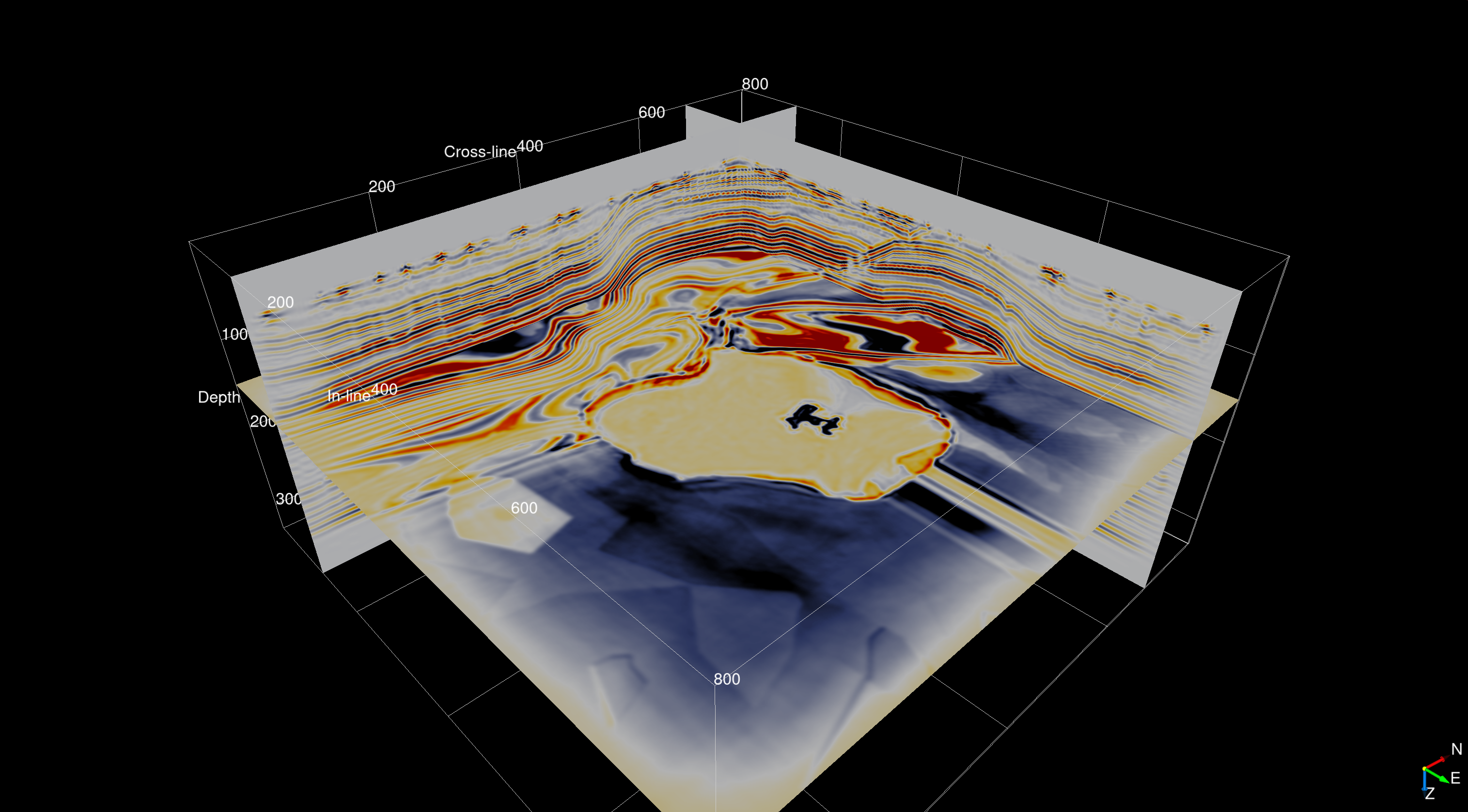
The subsurface velocity model used in this study is an artificial anisotropic model that is designed and built combining two broadly known and used open-source SEG/EAGE acoustic velocity models that each come with realistic geophysical imaging challenges such as sub-salt imaging. The anisotropy parameters are derived from a smoothed version of the velocity while the tilt angles were derived from a combination of the smooth velocity models and vertical and horizontal edge detection. The final seismic image of the subsurface model is displayed in Figure 1 and highlights the fact that 3D seismic imaging based on a serverless approach and automatic code generation is feasible and provides good results.

(P. A. Witte et al., 2020) describes the serverless implementation of seismic inverse problems in detail, including iterative algorithms for least-square minimization problems (LSRTM). The 3D anisotropic imaging results were presented as part of a keynote presentation at the EAGE HPC workshop in October 2019 (Herrmann et al., 2019) and at the Rice O&G HPC workshop (Witte et al., 2019a) in which the focus was on the serverless implementation of seismic inversion algorithms in the Cloud. This work illustrates the flexibility and portability of Devito: we were able to easily port a code developed and tested on local hardware to the Cloud, with only minor adjustments. Further, note that this experiment included the porting of MPI-based code for domain decomposition developed on desktop computers to the Cloud. Our experiments are reproducible using the instructions in a public repository AzureTTI, which contains, among the other things, the Dockerfiles and Azure batch-shipyard setup. This example can also be easily run on a traditional HPC cluster environment using, for example, JUDI (Witte et al., 2019b) or Dask (Rocklin, 2015) for parallelization over sources.
Elastic modelling
While the subsurface image obtained in section #d-imaging-example-on-azure utilized anisotropic propagators capable of mimicking intricate physics, in order to model both the wave kinematics and amplitudes correctly, elastic propagators are required. These propagators are, for example, extremely important in global seismology since shear surface waves (which are ignored in acoustic models) are the most hazardous. In this section, we exploit the tensor algebra language introduced in Devito v4.0 to express an elastic model with compact and elegant notation.
The isotropic elastic wave-equation, parametrized by the so-called Lamé parameters \(\lambda, \mu\) and the density \(\rho\) reads: \[ \begin{equation} \begin{aligned} &\frac{1}{\rho}\frac{dv}{dt} = \nabla . \tau \\ &\frac{d \tau}{dt} = \lambda \mathrm{tr}(\nabla v) \mathbf{I} + \mu (\nabla v + (\nabla v)^T) \end{aligned} \label{elas1} \end{equation} \] where \(v\) is a vector valued function with one component per cartesian direction: \[ \begin{equation} \begin{split} v = \begin{bmatrix} v_x(t, x, y) \\ v_y(t, x, y)) \end{bmatrix} \end{split} \label{partvel} \end{equation} \] and the stress \(\tau\) is a symmetric second-order tensor-valued function: \[ \begin{equation} \begin{aligned} \tau = \begin{bmatrix}\tau_{xx}(t, x, y) & \tau_{xy}(t, x, y)\\\tau_{xy}(t, x, y) & \tau_{yy}(t, x, y)\end{bmatrix}. \end{aligned} \label{stress} \end{equation} \] The discretization of Equation \(\ref{elas1}\) and \(\ref{stress}\) requires five equations in two dimensions (two equations for the particle velocity and three for the stress) and nine equations in three dimensions (three for the particle velocity and six for the stress). However, the mathematical definition only require two coupled vector/tensor-valued equations for any number of dimensions.
Tensor algebra language
We have augmented the Devito language with tensorial objects to enable straightforward and mathematically rigorous definitions of high-dimensional PDEs, such as the elastic wave-equation defined in \(\ref{elas1}\). This implementation was inspired by (Alnæs et al., 2014), a functional language for finite element methods.
The extended Devito language introduces two new types, VectorFunction/VectorTimeFunction for vectorial objects such as the particle velocity, and TensorFunction/TensorTimeFunction for second-order tensor objects (matrices) such as the stress. These new objects are constructed in the same manner as scalar Function objects. They also automatically implement staggered grid and staggered finite-differences with the possibility of half-node averaging. Each component of a tensorial object – a (scalar) Devito Function – is accessible via conventional vector notation (e.g. v[0],t[0,1]).
With this extended language, the elastic wave-equation defined in \(\ref{elas1}\) can be expressed in only four lines of code:
v = VectorTimeFunction(name='v', grid=model.grid, space_order=so, time_order=1)
tau = TensorTimeFunction(name='t', grid=model.grid, space_order=so, time_order=1)

u_v = Eq(v.forward, model.damp * (v + s/rho*div(tau)))
u_t = Eq(tau.forward,  model.damp *  (tau + s * (l * diag(div(v.forward)) + mu * (grad(v.forward) + grad(v.forward).T))))
The SymPy expressions created by these commands can be displayed with sympy.pprint as shown in Figure 2. This representation reflects perfectly the mathematics while maintaining computational portability and efficiency through the Devito compiler. The complete generated code for the elastic wave-equation with and without MPI is made available at CodeSample in elastic-so12.c and elastic-so12-mpi.c.

2D example
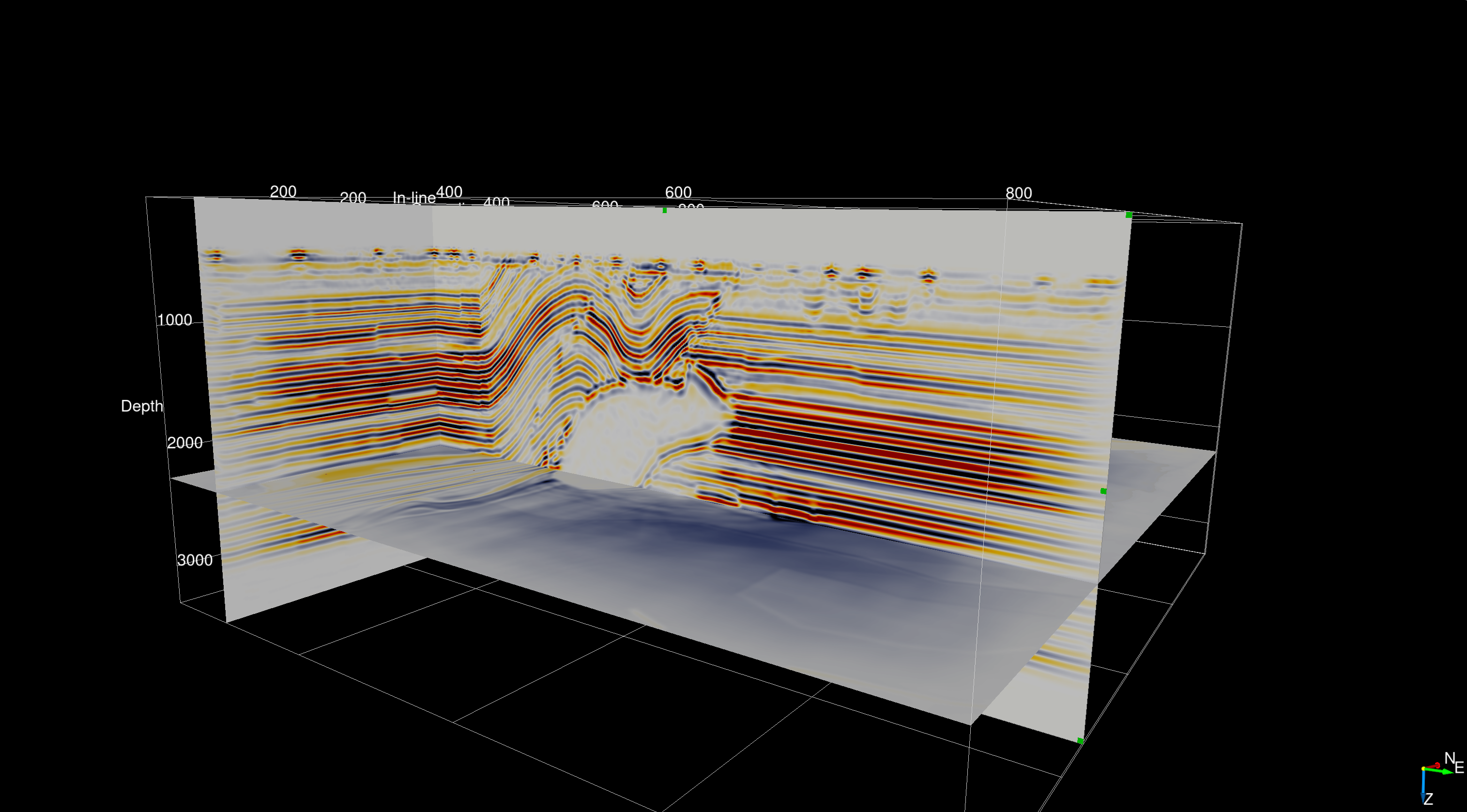
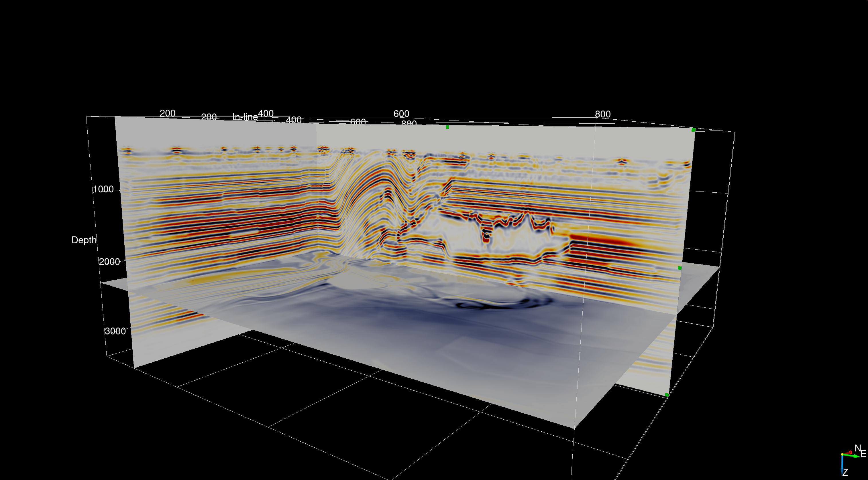
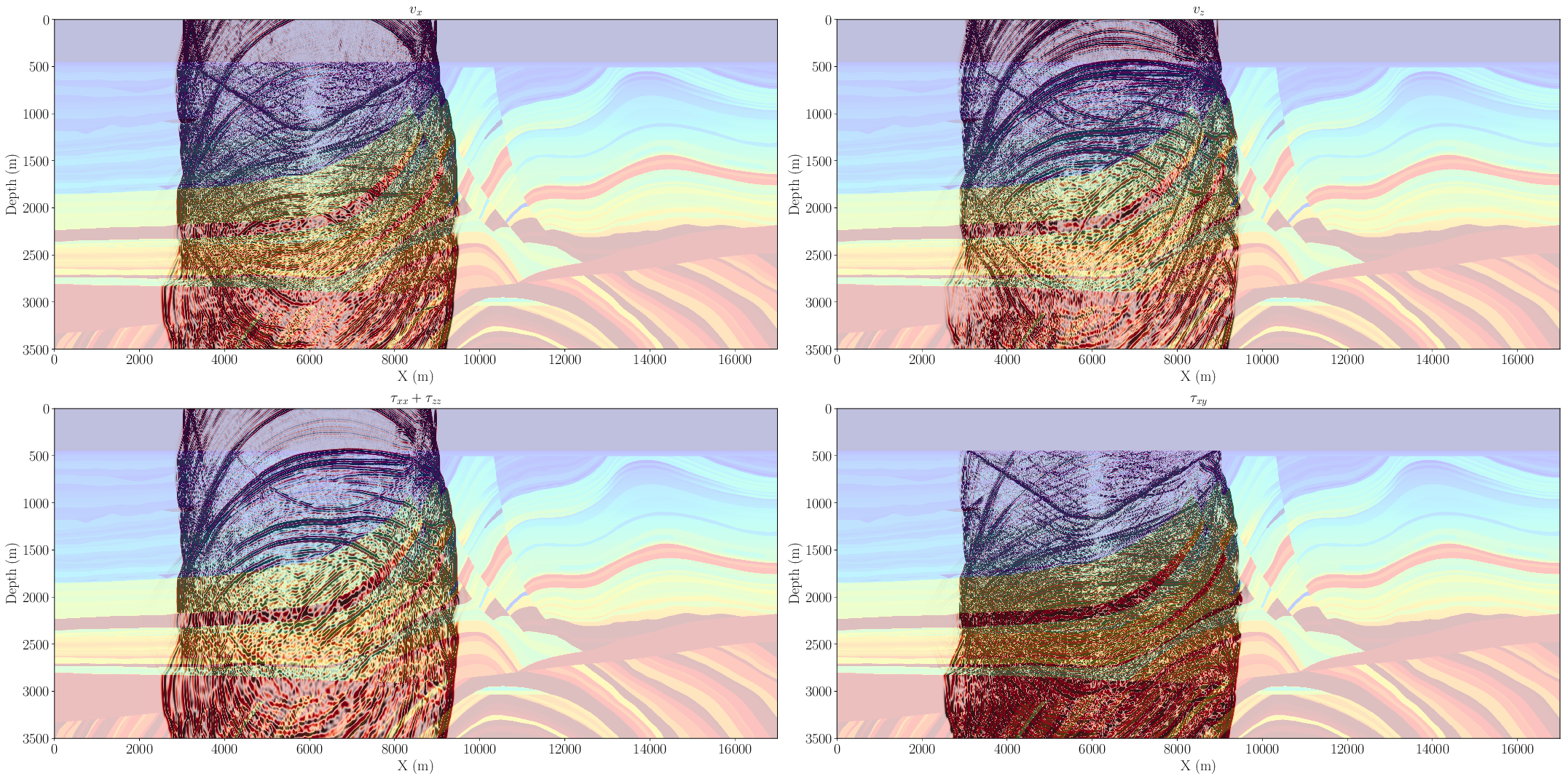
To demonstrate the efficacy of the elastic implementation outlined above we utilized a broadly recognized 2D synthetic model, the elastic Marmousi-ii(Versteeg, 1994; G. S. Martin et al., 2006) model. The wavefields are shown on Figure 3 and its corresponding elastic shot records are displayed in Figure 4. These two figures show that the wavefield is, as expected, purely acoustic in the water layer (\(\tau_{xy}=0\)) and transitions correctly at the ocean bottom to an elastic wavefield. We can also clearly see the shear wave-front in the subsurface (at a depth of approximately 1km). Figures 3 and 4 demonstrate that this high-level Devito implementation of the elastic wave-equation is effective and accurate. Importantly, in constructing this model within the Devito DSL framework, computational technicalities such as the staggered grid analysis are abstracted away. We note that the shot records displayed in Figure 4 match the original data generated by the creator of this elastic model (G. S. Martin et al., 2006).
x=5\text{km} in the marmousi-ii model.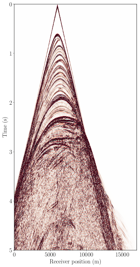
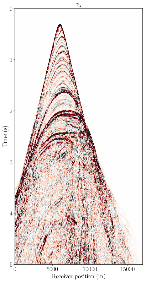

a is the pressure (trace of stress tensor) at the surface (5m depth), b is the vertical particle velocity and c is the horizontal particle velocity at the ocean bottom (450m depth).3D proof of concept
Finally, three dimensional elastic data was modelled in the Cloud to demonstrate the scalability of Devito to cluster-size problems. The model used in this experiment mimics a reference model in geophysics known as the SEAM model (Fehler and Keliher, 2011), a three dimensional extreme-scale synthetic representation of a subsurface. The physical dimensions of the model are 45kmx35kmx15km discretized with a grid spacing of 20mx20mx10m leading to a computational grid of 2250x1750x1500 grid points (5.9 billion grid points). One of the main challenges of elastic modelling is the extreme memory cost owing to the number of wavefields (a minimum of 21 fields in a three dimensional propagator) that need to be stored:
- Three particle velocities with two time steps (
v.forwardandv) - Six stress with two time steps (
tau.forwardandtau) - Three model parameters
lamda,muandrho
These 21 fields, for the 5.9 billion point grid defined above, lead to a minimum memory requirement of 461Gb for modelling alone. For this experiment, access was obtained for small HPC VMs (on Azure) called Standard_H16r. These VMs contain 16 core Intel Xeon E5 2667 v3 chips, with no hyperthreading, and 32 nodes were used for a single source experiment (i.e. a single wave-equation was solved). We used a 12th order discretization in space that led to 2.8TFLOP/time-step being computed by this model and the elastic wave was propagated for 16 seconds (23000 time steps). Completion of this modelling run took 16 hours, converting to 1.1TFLOP/s. While these numbers may appear low, it should be noted that the elastic kernel is extremely memory bound, while the TTI kernel is nearly compute bound (see rooflines in (Mathias Louboutin et al., 2017; M. Louboutin et al., 2019; Luporini et al., 2018)) making it more computationally efficient, particularly in combination with MPI. Future work will involve working on InfiniBand enabled and true HPC VMs on Azure to achieve Cloud performance on par with that of state of the art HPC clusters. Extrapolating from the performance obtained in this experiment, and assuming a fairly standard setup of 5000 independent source experiments, computing an elastic synthetic dataset would require 322 EFLOPs (23k time-steps x 2.8TFLOP/time-step x 5000 sources), or utilizing the full scalabilit
Performance comparison with other codes
Earlier performance benchmarks mainly focused on roofline model analysis. In this study, for completeness, the runtime of Devito is therefore compared to that of the open source hand-coded propagator fdelmodc. This propagator, described in (Thorbecke and Draganov, 2011), is a state of the art elastic kernel (Equation \(\ref{elas1}\)) and the comparisons presented here were carried out in collaboration with its author. To ensure a fair comparison, we ensured that the physical and computational settings were identical. The settings were as follows:
- 2001 by 1001 physical grid points.
- 200 grid points of dampening layer (absorbing layer (Cerjan et al., 1985)) on all four sides (total of 2401x1401 computational grid points).
- 10001 time steps.
- Single point source, 2001 receivers.
- Same compiler (gcc/icc) to compile fdelmodc and run Devito.
- Intel(R) Xeon(R) CPU E3-1270 v6 @ 3.8GHz.
- Single socket, four physical cores, four physical threads, thread pinning to cores and hyperthreading off.
The runtimes observed for this problem were essentially identical, showing less than a one percent of difference. Such similar runtimes were obtained with both the Intel and GNU compilers and the experiment was performed with both fourth and sixth order discretizations. Kernels were executed five times each and the runtimes observed were consistently very similar. This comparison illustrates the performance achieved with Devito is at least on par with hand-coded propagators. Considering we do not take advantage of the Devito compilers full capabilities in two dimensional cases, we are confident that the code generated will be at least on par with the hand-coded version for three dimensional problems and this comparison will be part of our future work.
Conclusions
Transitioning from academic toy problems, such as the two-dimensional acoustic wave-equation, to real-world applications can be challenging, particularly if this transition is carried out as an afterthought. Owing to the fundamental design principles of Devito such scaling, however, becomes trivial. In this work we demonstrated the high-level interface provided by Devito not only for simple scalar equations but also for coupled PDEs. This interface allows, in a simple, concise and consistent manner, the expression of all-kinds of non-trivial differential operators. Next, and most importantly, we demonstrated that the compiler enables large-scale modelling with state-of-the art computational performance and programming paradigm. The single-node performance is on par with state of the art hand-coded models, but packaged with this performance comes the flexibility of the symbolic interface and multi-node parallelism, which is integrated in the compiler and interface in a accessible way. Finally, we demonstrated that our abstractions provide the necessary portability to enable both on-premise and Cloud based HPC.
Code availability
The code to reproduce the different examples presented in this work is available online in the following repositories:
- The complete code for TTI imaging is available at Azure2019 and includes the TTI propagators, the Azure setup for shot parallelism and a documentation.
- The elastic modelling can be run with the elastic example available in Devito at elastic_example.py and can be run with any size and spatial order. A standalone script to run the large 3D elastic modelling is also available at codesamples
References
Alkhalifah, T., 2000, An acoustic wave equation for anisotropic media: Geophysics, 65, 1239–1250.
Alnæs, M. S., Logg, A., Ølgaard, K. B., Rognes, M. E., and Wells, G. N., 2014, Unified Form Language: A domain-specific language for weak formulations of partial differential equations: ACM Transactions on Mathematical Software (TOMS), 40, 9.
Baysal, E., Kosloff, D. D., and Sherwood, J. W. C. and, 1983, Reverse time migration: Geophysics, 48, 1514–1524.
Bube, K. P., Nemeth, T., Stefani, J. P., Ergas, R., Liu, W., Nihei, K. T., and Zhang, L., 2012, On the instability in second-order systems for acoustic vTI and tTI media: GEOPHYSICS, 77, T171–T186. doi:10.1190/geo2011-0250.1
Bube, K., Washbourne, J., Ergas, R., and Nemeth, T., 2016, Self-adjoint, energy-conserving second-order pseudoacoustic systems for vTI and tTI media for reverse time migration and full-waveform inversion: In SEG technical program expanded abstracts 2016 (pp. 1110–1114). SEG. doi:10.1190/segam2016-13878451.1
Bube*, K. P., Ergas, R., and Nemeth, T., 2014, Stability and energy conservation for second-order acoustic systems for vTI andTTI media with positive shear wavespeeds: In SEG technical program expanded abstracts 2014 (pp. 3439–3443). SEG. doi:10.1190/segam2014-0986.1
Cerjan, C., Kosloff, D., Kosloff, R., and Reshef, M., 1985, A nonreflecting boundary condition for discrete acoustic and elastic wave equations: GEOPHYSICS, 50, 705–708. doi:10.1190/1.1441945
Chu, C., Macy, B. K., and Anno, P. D., 2011, Approximation of pure acoustic seismic wave propagation in tTI media: GEOPHYSICS, 76, WB97–WB107. doi:10.1190/geo2011-0092.1
Duveneck, E., and Bakker, P. M., 2011, Stable p-wave modeling for reverse-time migration in tilted tI media: GEOPHYSICS, 76, S65–S75. doi:10.1190/1.3533964
Fehler, M., and Keliher, P. J., 2011, SEAM phase 1: Challenges of subsalt imaging in tertiary basins, with emphasis on deepwater gulf of mexico: Society of Exploration Geophysicists.
Fichtner, A., 2010, Full Seismic Waveform Modelling and Inversion: Springer Verlag. doi:10.1007/978-3-642-15807-0
Fletcher, R. P., Du, X., and Fowler, P. J., 2009, Reverse time migration in tilted transversely isotropic (tTI) media: GEOPHYSICS, 74, WCA179–WCA187. doi:10.1190/1.3269902
Fowler, P. J., Du, X., and Fletcher, R. P., 2010, Coupled equations for reverse time migration in transversely isotropic media: GEOPHYSICS, 75, S11–S22. doi:10.1190/1.3294572
Herrmann, F. J., Jones, C., Gorman, G., Hückelheim, J., Lensink, K., Kelly, P., … Witte, P. A., 2019, Accelerating ideation & innovation cheaply in the cloud the power of abstraction, collaboration & reproducibility: 4th eAGE workshop on high-performance computing.
Hooke, R., Papin, D., Sturmy, S., and Young, J., 1678, Lectures de potentia restitutiva: London : Printed for John Martyn ... Retrieved from http://lib.ugent.be/catalog/rug01:001559640
Köhn, D., Hellwig, O., De Nil, D., and Rabbel, W., 2015, Waveform inversion in triclinic anisotropic media—a resolution study: Geophysical Journal International, 201, 1642–1656. doi:10.1093/gji/ggv097
Krebs, J., Collis, S., Downey, N., Ober, C., Overfelt, J., Smith, T., … Young, J., 2014, Full wave inversion using a spectral-element discontinuous galerkin method:, 2014, 1–5. doi:https://doi.org/10.3997/2214-4609.20140707
Logg, A., Mardal, K.-A., Wells, G. N., and others, 2012, Automated solution of differential equations by the finite element method: Springer. doi:10.1007/978-3-642-23099-8
Louboutin, M., 2020, Modeling for inversion in exploration geophysics: PhD thesis,. Georgia Institute of Technology. Retrieved from https://slim.gatech.edu/Publications/Public/Thesis/2020/louboutin2020THmfi/louboutin2020THmfi.pdf
Louboutin, M., Lange, M., Herrmann, F. J., Kukreja, N., and Gorman, G., 2017, Performance prediction of finite-difference solvers for different computer architectures: Computers & Geosciences, 105, 148–157. doi:https://doi.org/10.1016/j.cageo.2017.04.014
Louboutin, M., Lange, M., Luporini, F., Kukreja, N., Witte, P. A., Herrmann, F. J., … Gorman, G. J., 2019, Devito (v3.1.0): An embedded domain-specific language for finite differences and geophysical exploration: Geoscientific Model Development, 12, 1165–1187. doi:10.5194/gmd-12-1165-2019
Louboutin, M., Witte, P. A., and Herrmann, F. J., 2018, Effects of wrong adjoints for rTM in tTI media: SEG technical program expanded abstracts. doi:10.1190/segam2018-2996274.1
Luporini, F., Lange, M., Louboutin, M., Kukreja, N., Hückelheim, J., Yount, C., … Herrmann, F. J., 2018, Architecture and performance of devito, a system for automated stencil computation: CoRR, abs/1807.03032. Retrieved from http://arxiv.org/abs/1807.03032
Lyu, C., Capdeville, Y., and Zhao, L., 2020, Efficiency of the spectral element method with very high polynomial degree to solve the elastic wave equation: GEOPHYSICS, 85, T33–T43. doi:10.1190/geo2019-0087.1
Martin, G. S., Wiley, R., and Marfurt, K. J., 2006, Marmousi2: An elastic upgrade for marmousi: The Leading Edge, 25, 156–166. doi:10.1190/1.2172306
Meurer, A., Smith, C. P., Paprocki, M., Čertík, O., Kirpichev, S. B., Rocklin, M., … Scopatz, A., 2017, SymPy: Symbolic computing in python: PeerJ Computer Science, 3, e103. doi:10.7717/peerj-cs.103
Patterson, D. A., and Hennessy, J. L., 2007, Computer organization and design: The hardware/Software interface: (3rd ed.). Morgan Kaufmann Publishers Inc.
Peter, D., Komatitsch, D., Luo, Y., Martin, R., Le Goff, N., Casarotti, E., … Tromp, J., 2011, Forward and adjoint simulations of seismic wave propagation on fully unstructured hexahedral meshes: Geophysical Journal International, 186, 721–739. doi:10.1111/j.1365-246X.2011.05044.x
Petersson, N., and Sjögreen, B., 2014, SW4 v1.1 [software]: Computational Infrastructure for Geodynamics. doi:http://doi.org/10.5281/zenodo.571844
Preston, L., 2018, Computation of kernels for full waveform seismic inversion using parelasti.:. doi:10.2172/1468379
Preston, L., 2019a, Paraniso 1.0: 3-d full waveform seismic simulation in general anisotropic media.:. doi:10.2172/1561580
Preston, L., 2019b, ParelastiFWI 1.0 user guide.:. doi:10.2172/1561581
Ratcliffe, A., Win, C., Vinje, V., Conroy, G., Warner, M., Umpleby, A., … Bertrand, A., 2011, Full waveform inversion: A north sea OBC case study: SEG Technical Program Expanded Abstracts 2011. doi:10.1190/1.3627688
Rathgeber, F., Ham, D. A., Mitchell, L., Lange, M., Luporini, F., McRae, A. T. T., … Kelly, P. H. J., 2015, Firedrake: Automating the finite element method by composing abstractions: CoRR, abs/1501.01809. Retrieved from http://arxiv.org/abs/1501.01809
Rocklin, M., 2015, Dask: Parallel computation with blocked algorithms and task scheduling: In K. Huff & J. Bergstra (Eds.), Proceedings of the 14th python in science conference (pp. 130–136).
Sirgue, L., I. Barkved, O., P. Van Gestel, J., J. Askim, O., and H. Kommedal, J., 2009, 3D waveform inversion on valhall wide-azimuth oBC:. doi:https://doi.org/10.3997/2214-4609.201400395
Tarantola, A., 1984, Inversion of seismic reflection data in the acoustic approximation: GEOPHYSICS, 49, 1259. doi:10.1190/1.1441754
Thomsen, L., 1986, Weak elastic anisotropy: Geophysics, 51, 1964–1966.
Thorbecke, J. W., and Draganov, D., 2011, Finite-difference modeling experiments for seismic interferometry: GEOPHYSICS, 76, H1–H18. doi:10.1190/geo2010-0039.1
Trinh, P.-T., Brossier, R., Métivier, L., Tavard, L., and Virieux, J., 2019, Efficient time-domain 3D elastic and viscoelastic full-waveform inversion using a spectral-element method on flexible cartesian-based mesh: Geophysics, 84, R75–R97.
Versteeg, R., 1994, The marmousi experience; velocity model determination on a synthetic complex data set: The Leading Edge, 13, 927–936. Retrieved from http://tle.geoscienceworld.org/content/13/9/927
Virieux, J., and Operto, S., 2009, An overview of full-waveform inversion in exploration geophysics: GEOPHYSICS, 74, WCC1–WCC26. doi:10.1190/1.3238367
Virieux, J., Operto, S., Ben-Hadj-Ali, H., Brossier, R., Etienne, V., Sourbier, F., … Haidar, A., 2009, Seismic wave modeling for seismic imaging: The Leading Edge, 28, 538–544. doi:10.1190/1.3124928
Whitmore, N. D., 1983, Iterative depth migration by backward time propagation: 1983 SEG Annual Meeting, Expanded Abstracts.
Witte, P. A., Louboutin, M., Jones, C., and Herrmann, F. J., 2019a, Serverless seismic imaging in the cloud: Retrieved from https://slim.gatech.edu/Publications/Public/Submitted/2019/witte2019RHPCssi/witte2019RHPCssi.html
Witte, P. A., Louboutin, M., Kukreja, N., Luporini, F., Lange, M., Gorman, G. J., and Herrmann, F. J., 2019b, A large-scale framework for symbolic implementations of seismic inversion algorithms in julia: Geophysics, 84, F57–F71. doi:10.1190/geo2018-0174.1
Witte, P. A., Louboutin, M., Modzelewski, H., Jones, C., Selvage, J., and Herrmann, F. J., 2019c, Event-driven workflows for large-scale seismic imaging in the cloud: SEG technical program expanded abstracts. doi:10.1190/segam2019-3215069.1
Witte, P. A., Louboutin, M., Modzelewski, H., Jones, C., Selvage, J., and Herrmann, F. J., 2020, An event-driven approach to serverless seismic imaging in the cloud:IEEE Transactions on Parallel and Distributed Systems. IEEE.
Witte, P. A., Stolk, C. C., and Herrmann, F. J., 2016, Phase velocity error minimizing scheme for the anisotropic pure p-wave equation: SEG technical program expanded abstracts. doi:10.1190/segam2016-13844850.1
Xu, S., and Zhou, H., 2014, Accurate simulations of pure quasi-p-waves in complex anisotropic media: Geophysics, 79, 341–348.
Zehner, B., Hellwig, O., Linke, M., Görz, I., and Buske, S., 2016, Rasterizing geological models for parallel finite difference simulation using seismic simulation as an example: Computers & Geosciences, 86, 83–91. doi:https://doi.org/10.1016/j.cageo.2015.10.008
Zhan, G., Pestana, R. C., and Stoffa, P. L., 2013, An efficient hybrid pdeudospectral/finite-difference scheme for solving the tTI pure p-wave equation: Journal of Geophyics and Engineering, 10.
Zhang, L., Rector III, J. W., and Micheal, H. G., 2005, Finite-difference modelling of wave propagation in acoustic tilted tI media: Geophysical Prospecting, 53, 843–852.
Zhang, Y., Zhang, H., and Zhang, G., 2011, A stable tTI reverse time migration and its implementation: GEOPHYSICS, 76, WA3–WA11. doi:10.1190/1.3554411
Zhang, Y., Zhang, H., and Zhang, G., 2011, A stable tTI reverse time migration and its implementation: Geophysics, 76, WA3–WA11.