Joint full-waveform inversion of on-land surface and VSP data from the Permian Basin

Brendan R. Smithyman^*, Bas Peters^*, Bryan DeVault^† and Felix J. Herrmann^*
*Seismic Laboratory for Imaging and Modeling (SLIM), The University of British Columbia
^†Vecta Oil and Gas, Inc.

Case study

The “Near Miss” dataset was acquired by Vecta Oil and Gas in 2010 to image Lower Paleozoic transpressional pop-up structures prospective for oil and gas in the Permian Basin of Texas, USA. The recorded data include well logs and seismic waveforms from two surveys that were acquired concurrently:

1. a 3-D VSP survey comprising 2787 surface vibroseis sources and 151 downhole 3-component geophones; and,
2. a 3-D seismic reflection survey comprising 2831 vibroseis sources and 1649 vertically-polarised geophones.

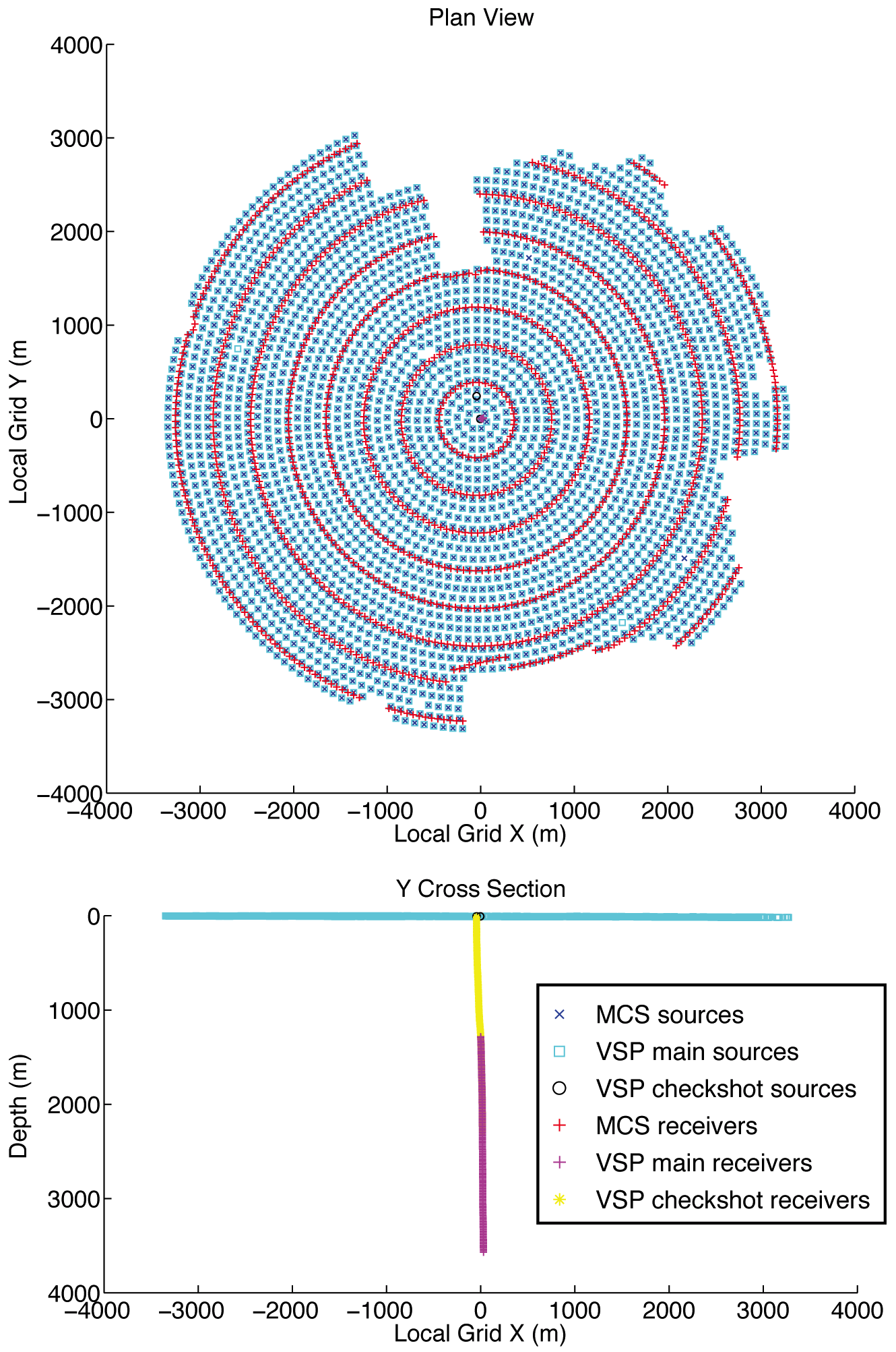
Of the vibration points that were shot, 2785 were common to both surveys; Figure 1 shows the acquisition geometry, including the receivers for both arrays and the common sources that were processed in joint inversion. The surface sources and receivers were placed in equally-spaced concentric rings surrounding the central VSP well. The top VSP geophone was emplaced at 1.3 km depth and the bottom geophone was emplaced at 3.6 km depth. The source vibroseis sweep contained frequencies from 8–120 Hz, and the surface geophones were critically damped above 10 Hz, whereas the downwell geophones were critically damped above 15 Hz. This yielded a practical starting frequency for FWI of 8 Hz, with maximal Signal to Noise Ratio (SNR) at about 10 Hz. Several checkshot sweeps were also recorded before the VSP array was installed at depth; these provide information about the near-surface 1D velocity structure that was used in the development of the initial velocity model; however, these data were not inverted during FWI.

The initial velocity model used by joint FWI was developed by industry contractors during Pre-Stack Depth Migration (PSDM) processing. It represents a smooth estimate of the vertical P-wave velocity based on checkshot velocities recorded in the central VSP well and variability determined by 3-D Migration Velocity Analysis (MVA). The initial migrated image provided sufficient detail to focus reflectors effectively to middle depths, but lensing through high-velocity carbonate rocks at 1200–2700 m depth resulted in mis-migration at reservoir depths. This motivates full-waveform processing to improve the quality of the velocity model.

Methodology

Full-waveform Inversion is a nonlinear process by which an Earth model is iteratively updated to better predict recorded field seismograms. The full-waveform inversion procedure we follow herein is based on Herrmann et al. (2013) and Pratt (1999), but with several adaptations to enable the processing of 3-D on-land field data using a 2-D acoustic FWI code. The numerical implementation is developed in Parallel MatLab and allows for parallelism over frequencies. \[ \begin{equation} \label{helmholtz} \left[L + \omega^2\text{diag}\left(\mathbf{x}\right)\right]\mathbf{u} = \mathbf{q} + \text{BCs} \end{equation} \] where \(L\) is the discrete Laplacian operator, \(\omega\) is the angular frequency, \(\mathbf{x}\) is the model, \(\mathbf{q}\) is the source signature and \(\mathbf{u}\) is the pressure field. The inversion procedure updates the model of squared slowness, \(\mathbf{x} = \frac{1}{\mathbf{c}^2}\). The Field seismograms are the result of waves propagating in three dimensions, through a complex elastic earth, whereas the simulated seismograms from our method represent solutions to the 2-D constant-density Helmholtz equation (Equation \(\ref{helmholtz}\)).

The joint inversion of the MCS and VSP datasets results in equivalent but separate processing steps at several stages of the inversion. A number of practical choices are made to improve the tractability of the FWI problem, which are discussed here. Several 2-D cross-sectional slices are processed by independent 2-D FWI, though the resulting models are assessed together; these separate FWI problems use appropriate subsets of the sources and receivers from the 3-D survey, and do not share data or depend on each other.

Sources and receivers are modelled using dipoles oriented vertically, in order to account approximately for the radiation and sensitivity patterns expected from the vibroseis sources and vertically-polarised geophones. The source signature is estimated by Newton search based on the data residuals corresponding to the current model iterate at each stage of inversion. A separate calibration factor is computed for each array (viz., the MCS and VSP receivers) to account automatically for their differing geophone responses. The bulk Amplitude Variation with Offset (AVO) characteristics of the medium are scaled to account partially for the differing geometric spreading patterns between the 3-D elastic Earth and the 2-D acoustic medium that is modelled. This is accommodated by a log-linear AVO scale factor (see Brenders & Pratt, 2007; B. R. Smithyman & Clowes, 2012), which is determined independently for each dataset in joint inversion.

The l-BFGS quasi-Newton method (Nocedal & Wright, 2000) is used to minimize the unconstrained problem in Equation \(\eqref{objective}\), which improves convergence rates in comparison with a projected gradient method. The data misfit function is augmented by a model-dependent (Tikhonov) smoothness-regularization term (Equation \(\ref{roughening}\)) that is computed by a 2-D wavenumber high-pass filter. This penalizes features in the model iterate that are supported by high spatial wavenumbers. This approximates the effects of a wavenumber filtering approach that is sometimes used with projected gradient solvers (Pratt, 1999; Song, Williamson, & Pratt, 1995).

The roughening operator is defined, \[ \begin{equation} \label{roughening} R = E^* F^* S F E \end{equation} \] where \(E\) and \(F\) are linear operators that perform mirror extension and the 2-D Fast Fourier Transform (FFT), respectively, \(S\) is a selection matrix with diagonal values bounded on \(0 \leq s_i \leq 1\) and zeros elsewhere, and \({}^*\) denotes the complex conjugate transpose. The values of \(s_i\) are chosen to select an ellipsoidal region around the zero wavenumber in Fourier space with value \(1\) and a second ellipsoidal region centred on the zero wavenumber but of larger size, outside of which the values are set to \(0\). The values between are tapered to generate a smooth 2D frequency-domain filter. The roughening operator enters as a model-dependent term in the objective function (Equation 3): \[ \begin{equation} \label{objective} E = \frac{1}{2} \left[\|\mathcal{A}\left(\mathbf{x}\right) - \mathbf{b}\|_2^2 + \lambda_1 \|R\mathbf{x}\|_2^2 + \lambda_2 \|D\left(\mathbf{x} - \mathbf{x}_0\right)\|_2^2 \right] \end{equation} \] with \(\mathbf{x}\) representing the model vector, \(\mathbf{b}\) representing the data vector, and \(\mathcal{A}\) representing a nonlinear map that generates forward-modeled data given \(\mathbf{x}\). The reference model term \(D\) is a diagonal matrix bounded on \([0,1]\) that penalizes deviation from an a priori reference model \(\mathbf{x}_0\) (conventionally taken to be the starting model). The scalar multipliers \(\lambda_1\), \(\lambda_2\) determine the strength of the smoothness and reference-model quadratic penalty terms.

The objective function is regularized to favour smooth models by penalizing the high wavenumbers. The filter coefficients for the construction of \(R\) are chosen adaptively, such that the vertical wavenumbers in the model are limited above a scaled threshold \(k_{max} = \frac{\omega_{max}}{c_{min}}\) at each iteration. The horizontal wavenumber limit is chosen in terms of some ratio to the vertical wavenumber limit (typically ~5:1) in order to encourage models that exhibit strong horizontal smoothness; this is representative of the expected structures in a sedimentary basin such as the Permian Basin. The wavenumber content of the model constraint is adapted based on the temporal frequencies included at each stage of the FWI procedure; hence, structures in the model are tied to some proportion of the theoretical resolving power of the FWI sensitivity kernel (see Wu & Toksöz, 1987) for the maximum frequency at each iteration.

Because the accurate modelling of the physics is highly dependent on the initial velocity model, a poor choice of initial model will cause the inversion to converge towards a local minimum of the objective function far from the global minimum (Pratt, 1999; Shah, Warner, Guasch, Štekl, & Umpleby, 2010). We therefore assess the initial data misfit for both datasets considered by joint inversion. Particular attention is paid to the phase misfit, which depends strongly on the kinematics of the waves and may be examined to determine whether the model under- or over-predicts traveltimes by more than one half cycle. If the phase misfit for given source/receiver pair is larger than a half cycle then the FWI process may converge towards a local minimum of the objective function (Shah et al., 2010).

Results

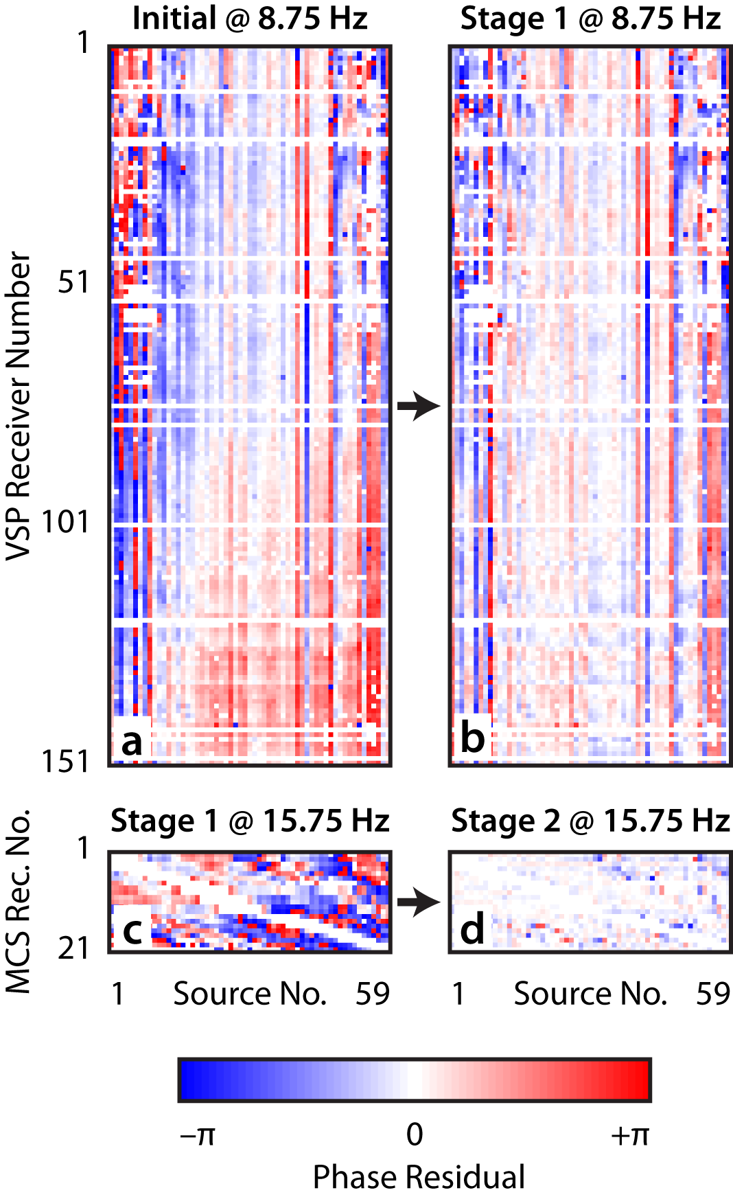
Examination of the data misfit for the VSP data in the initial velocity model (Figure 2a) indicates that the phase residuals are universally less than one half cycle (i.e., +/- pi; see Figure 3a) at the starting frequency of 8 Hz. This is straightforward to assess because the spatial sampling of the sources at surface (~107 m) and in the VSP well (~17 m) are sufficiently fine to preclude spatial aliasing at the lowest velocity present in the model (~2500 m/s). However, because the surface receivers are sampled much more coarsely (~402 m), it is difficult to assess whether cycle skips are present in residuals for the MCS array (e.g., by visual artefacts; see Shah et al. (2010)). Consequently, our methodology uses only the surface sources and VSP receivers for the first stage of FWI, which includes frequencies from 8–9 Hz. The data from the MCS array are introduced in the second stage of inversion, with the expectation that the near-surface part of the model sampled by both arrays will not produce cycle skips in the MCS data residuals after the updates from the first stage of FWI.

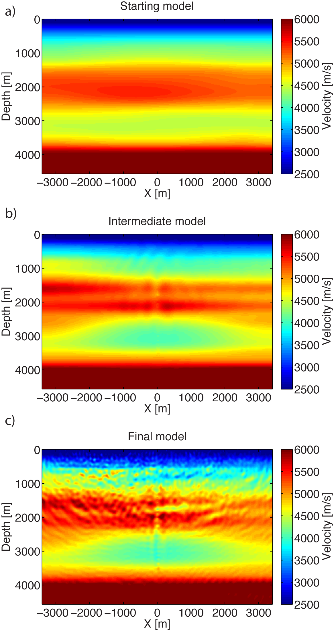
Figure 2 shows the models of P-wave velocity at different stages of the FWI procedure. The application of the first stages of FWI resulted in an improved model of P-wave velocity that substantially reduced the phase misfit for the VSP array; cf. Figure 3 a and b. The model resulting from the first stage of FWI (Figure 2b) possesses similar wavenumber content to the initial model (produced during MVA; Figure 2a), but exhibits layered low- and high-velocity features that correspond with prior ground truth from the sonic logs. The thickness of the middle-depth high-velocity layer is preserved in the centre of the model (near \(x=0\)), but the FWI updates produce a thicker high-velocity region towards the western end of the model.

A second stage of FWI incorporates data from the surface MCS survey, and jointly inverts these data along with the data waveforms from the VSP survey. The source modelling is the same for both arrays, but the surface dataset is weighted by a scalar to produce a total data misfit on the same order of magnitude as the corresponding data misfit from the VSP array. Unlike the data from the VSP survey, the MCS data are not sufficiently well-sampled by the geophones to avoid spatial aliasing, which is one motivation for imposing smoothness regularization in the objective function (Equation \(\ref{objective}\)).

The second stage of FWI was carried out using frequencies from 8 Hz to 15.75 Hz, which resulted in substantially-reduced smoothing because of the frequency-dependent bounds for the wavenumber regularization filter. The data misfit is reduced substantially for both the VSP and MCS arrays (see misfit reduction for MCS data, Figure 3c and d). The model updates resulting from the second stage (Figure 2c) identify raised topography in the centre of the model, with anticlinal features that are unconformably overlain by flat-lying features with an increased P-wave velocity. The high-velocity layer at middle depths possesses significantly different P-wave velocities than the layers above and below, and the characterization of its shape is critical for successful migration of rocks underlying it.

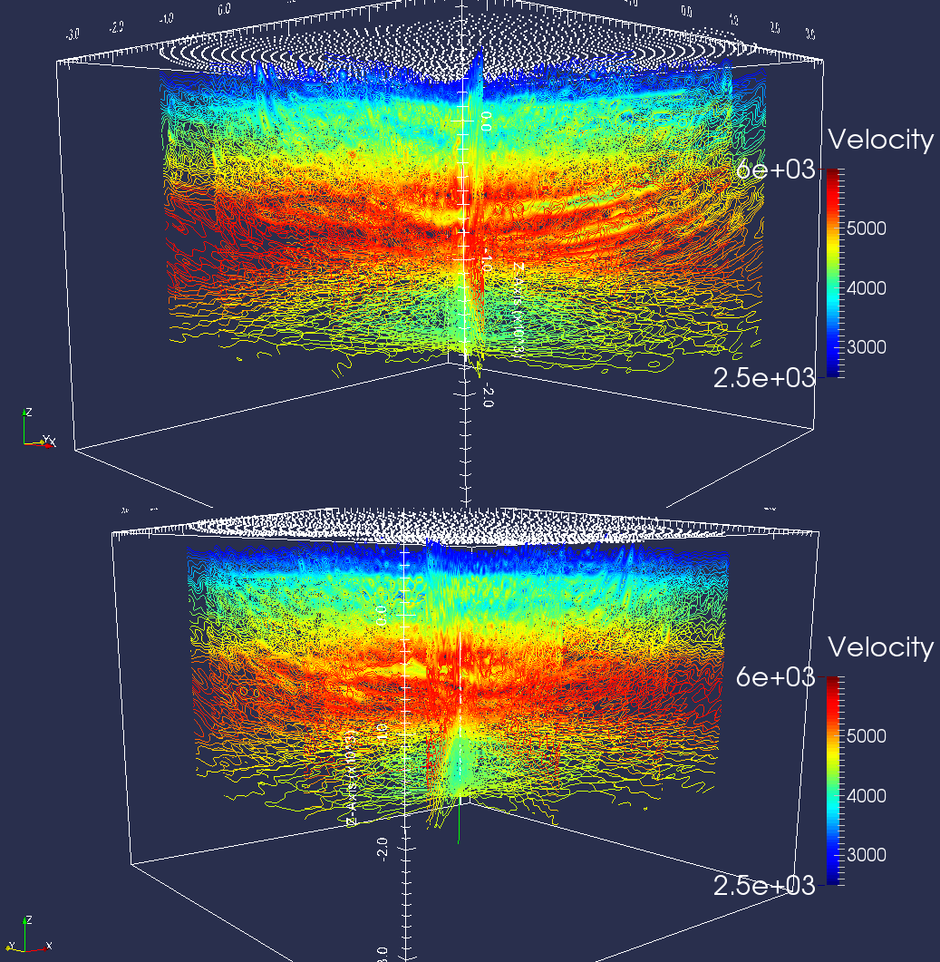
Due to the complexity of the site used in this case study and the high data frequencies, 3-D FWI has not yet been applied to this dataset. However, a series of eight 2-D cross-sectional models has been produced from the application of this 2-D FWI workflow at intervals of 22.5° North azimuth; see Figure 4. These show good agreement in the central (overlapping) region of the site, and illuminate 3-D structures at a moderate additional computational cost (\(8\times\) the cost of a single 2-D profile). Because of the level of automation present in our workflow, parameter tuning is carried out once and minimal additional operator time is required to process these additional profiles.

Discussion and Conclusions

The application of joint Full-Waveform Inversion (FWI) to land data from multichannel seismic (MCS) and vertical seismic profiling (VSP) arrays represents a challenging imaging exercise. The velocity models that are recovered provide improved detail over models generated by conventional migration velocity analysis; this improvement comes from iterative inversion of the data waveforms. The automatic pre-stack application of this method to un-processed field waveforms avoids the hands-on approach that is typical of a conventional seismic imaging workflow. It is perhaps worth emphasizing that the data from this case study are processed semi-automatically from the raw field records, without manual manipulation of the waveforms and starting at minimum vibroseis sweep frequency of 8 Hz.

Reverse-Time Migration is applied in the pre-stack workflow to image the high-wavenumber structures that are not present in the smooth seismic velocity model. The nonlinearity present in the full-waveform inversion problem necessitates a high-quality initial model of P-wave velocity. In most workflows, the natural source for this initial model would be conventional migration velocity analysis; hence, the FWI step is positioned to produce iterative improvements on preexisting MVA models.

The use of refracted data waveforms recorded on both MCS and VSP arrays potentially enables the recovery of detailed velocity models for a substantial part of the depth range; this can greatly benefit later pre-stack depth migration. However, since the model of velocity is updated using refraction waveforms that are not typically used in inversion, it is important to pay attention to the differing sensitivities between the near-vertical migration wavepaths and the sub-horizontal wavepaths used in FWI. In particular, the models of P-wave velocity from FWI may not be directly applicable for migration in the presence of strong anisotropy. If the vertical propagation velocity is very different from the horizontal propagation velocity then the use of anisotropic FWI and migration algorithms may result in mis-positioning of reflectors. A general application of joint FWI for surface and VSP datasets will require consideration of the effects of anisotropy.

The application of a true 3-D processing workflow for FWI is computationally challenging, benefits from several advantages when dealing with field data:

1. the geometric-spreading behaviour of the numerical modelling matches much more closely the field data, which enables improved processing and inversion of the data amplitudes;
2. the illumination of targets from a wide range of angles substantially improves the quality of the imaging and inversion results.

Our current research involves the application of 2-D and 3-D processing to this dataset, in the pursuit of a high-resolution 3-D model of subsurface velocity that may be used to substantially improve on existing 3-D prestack depth migration images.

Acknowledgments

This work was financially supported in part by the Natural Sciences and Engineering Research Council of Canada Discovery Grant (RGPIN 261641-06) and the Collaborative Research and Development Grant DNOISE II (CDRP J 375142-08). This research was carried out as part of the SINBAD II project with support from the following organizations: BG Group, BGP, BP, Chevron, ConocoPhillips, CGG, ION GXT, Petrobras, PGS, Statoil, Total SA, WesternGeco, and Woodside. Vecta Oil and Gas provided the “Near Miss” dataset. The authors would like to thank Morgan Brown of Wave Imaging Technology, who carried out initial PSDM processing and Andres Chavarria of SR2020, who processed the VSP data.

References

Brenders, A., & Pratt, R. G. (2007). Full waveform tomography for lithospheric imaging: results from a blind test in a realistic crustal model. Geophysical Journal International, 168(1), 133–151.
Herrmann, F. J., Hanlon, I., Kumar, R., Leeuwen, T. van, Li, X., Smithyman, B., … Takougang, E. T. (2013). Frugal full-waveform inversion: From theory to a practical algorithm. The Leading Edge, 32(9), 1082–1092.
Nocedal, J., & Wright, S. J. (2000). Numerical optimization. Springer.
Pratt, R. G. (1999). Seismic waveform inversion in the frequency domain, Part 1: Theory and verification in a physical scale model. Geophysics, 64(3), 888–901.
Shah, N., Warner, M., Guasch, L., Štekl, I., & Umpleby, A. P. (2010). Waveform inversion of surface seismic data without the need for low frequencies. SEG 2010 Annual Meeting, 2865–2869.
Smithyman, B. R., & Clowes, R. M. (2012). Waveform tomography of field vibroseis data using an approximate 2D geometry leads to improved velocity models. Geophysics, 77(1), R33–R43.
Song, Z. M., Williamson, P. R., & Pratt, R. G. (1995). Frequency-domain acoustic wave modeling and inversion of crosshole data: Part II–Inversion method, synthetic experiments and real-data results. Geophysics, 60(3), 796–809.
Wu, R., & Toksöz, M. (1987). Diffraction tomography and multisource holography applied to seismic imaging. Geophysics, 52(1), 11–25.