Neural Operators with Accurate Jacobian for High-Fidelity Image-Domain Seismic Inversion
1 Introduction
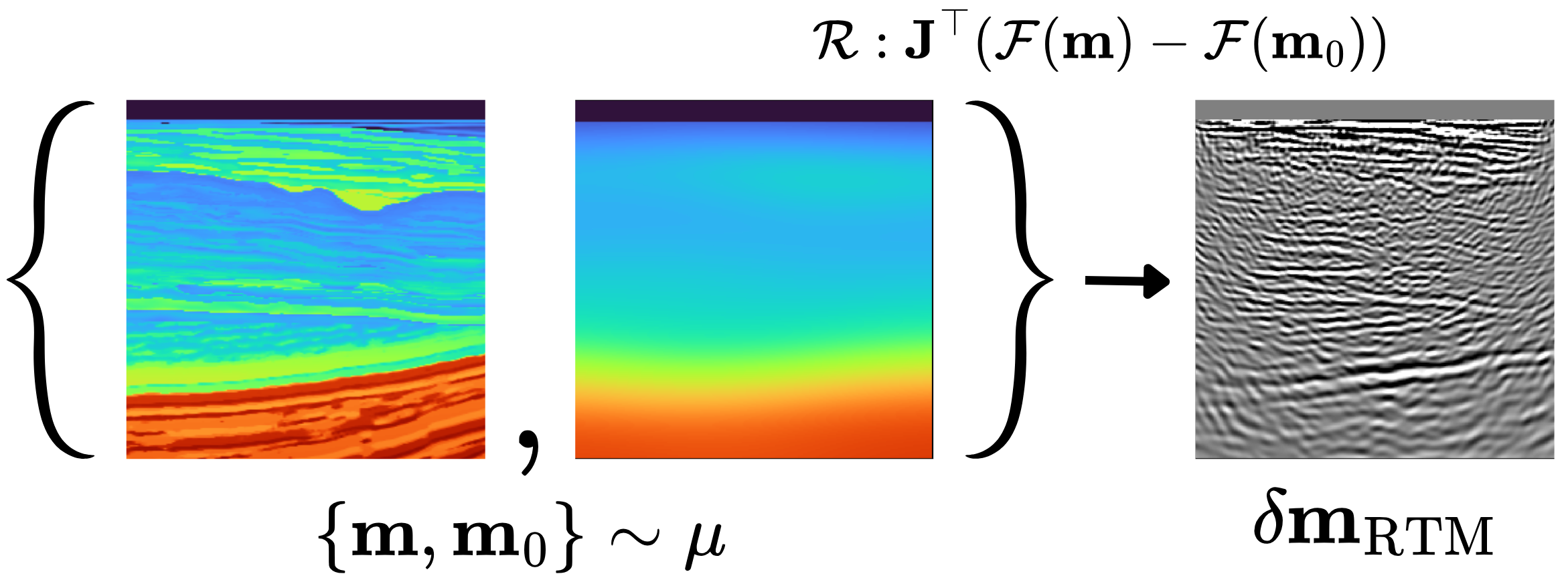
In seismic inversion, Image-Domain Least-Squares Migration (IDLSM) constructs subsurface images by solving a linearized inverse problem based on the Born modeling operator and its adjoint (Symes 2008). While producing high-resolution subsurface images, these methods remain computationally expensive due to repeated large-scale wave-equation solves, with cost scaling with acquisition size (Tarantola 1984; Virieux and Operto 2009; Louboutin et al. 2017). To mitigate these costs, recent work has explored Machine Learning approaches that accelerate components of the seismic imaging workflow (Geng et al. 2022; Orozco et al. 2024; Yin et al. 2024; Yin, Orozco, and Herrmann 2025; Erdinc et al. 2025). In this work, we train a neural surrogate for a nonlinear, image-domain operator induced by migration. Specifically, we approximate an imaging operator that maps subsurface and background-velocity models to an RTM image: \[ \mathcal{R}: (\mathbf{m}, \mathbf{m}_0) \mapsto \delta \mathbf{m}_{\mathrm{RTM}}, \tag{1}\] where \(\mathbf{m}\), \(\mathbf{m}_0\) and \(\delta \mathbf{m}_{\mathrm{RTM}}\) are the subsurface velocity model, smooth background-velocity model and the migrated image, respectively. We approximate this mapping using neural operators, which learn mappings between function spaces governed by PDEs (Kovachki et al. 2023; Li et al. 2020). Once trained, these surrogates enable fast foward prediction and gradient computation via automatic differentiation (Siahkoohi, Louboutin, and Herrmann 2022; Ma and Alkhalifah 2025), replacing the numerical simulator and potentially providing efficient Gauss–Newton approximations for preconditioning.
However, accurate forward prediction alone does not ensure that the learned operator captures the derivative information required for inversion (Park, Yang, and Chandramoorthy 2024; Rosofsky, Al Majed, and Huerta 2023; Li et al. 2024; O’Leary-Roseberry et al. 2024; Park et al. 2025). Since gradient-based updates are governed by the adjoint Jacobian (Tarantola 1984; Virieux and Operto 2009), errors in the learned sensitivities lead to inaccurate gradients, unphysical updates, and degraded reconstruction quality (see rightmost column of Figure 5). This highlights the need to incorporate inversion-relevant sensitivity information during training.
To address this limitation, we introduce a Jacobian-informed training strategy that incorporates sensitivity information from Least-Squares Migration. Specifically, we supervise the neural operator along a small number of well-illuminated directions in model space, obtained from the dominant eigenvectors of the Gauss–Newton Hessian averaged over the training distribution. This yields a set of globally informative directions that capture the dominant sensitivity structure of the inverse problem. We further construct a dataset with variability in both subsurface and background-velocity models to enable inversion-oriented learning. Numerical experiments with Fourier Neural Operators (FNOs) (Li et al. 2020) show that the proposed approach produces more physically-aligned gradients, leading to improved recovery of subsurface velocity structures and reduced artifacts compared to standard training algorithm.
2 Theory: Informative Directions for Inversion
In the following subsections, we define the forward problem and identify directions that drive gradient-based inversion.
2.1 Linearized Modeling and RTM
Let \(\mathbf{m}\) define the discretized subsurface velocity model. When the forward operator, \(\mathcal{F}\), is linearized around a background model \(\mathbf{m}_0\) and \(\mathbf{d}_\text{obs}\) is seismic data, the RTM image at \(\mathbf{m}_0\) is \[\delta \mathbf{m}_{\mathrm{RTM}} = \mathbf{J}(\mathbf{m}_0)^\top (\mathcal{F}(\mathbf{m}_0) - \mathbf{d}_\text{obs}),\] where \(\mathbf{J}(\mathbf{m}_0)\) denotes the Born modeling operator.
2.2 Direction of gradient descents during inversion
During gradient-based seismic inversion, not all directions in the model space are equally constrained by the data (Tarantola 1984; Virieux and Operto 2009), due to limited acquisition geometry and band-limited sources. As a result, when performing gradient descent without additional prior information (e.g., maximum likelihood estimation), only a subset of model perturbations, which coincides with as well-illuminated directions, can be reliably recovered. That is, in Least-Squares Migration (LSM), the objective function and its gradient are given by \[ \begin{aligned} \mathcal{L}(\mathbf{m}) &= \frac{1}{2}\|\mathcal{R}(\mathbf{m}) - \delta \mathbf{m}_\mathrm{RTM} \|^2_2 \\ \nabla_\mathbf{m} \mathcal{L}(\mathbf{m}) &= \Bigl(\frac{\partial \mathcal{R}(\mathbf{m})}{\partial \mathbf{m}} \Bigr)^\top \mathbf{r}(\mathbf{m}) \end{aligned} \] where \(\mathbf{r}(\mathbf{m}) = \mathcal{R}(\mathbf{m}) - \delta \mathbf{m}_\mathrm{RTM}.\) The curvature of this objective function, which characterizes how perturbations in the model affect the data misfit and therefore which components of the model can be reliably recovered, is characterized by the Gauss–Newton Hessian (GNH), \[ \mathbf{H}_\text{GN}(\mathbf{m}) = \mathbf{J}(\mathbf{m})^\top\mathbf{J}(\mathbf{m}).\] To identify the shared directions that primarily drive inversion updates across varying models, we compute the dominant eigenvectors of the Gauss-Newton Hessian, \[ \begin{aligned} &\bar{\mathbf{H}}_\text{GN} = \mathbb{E}_\mu \Bigl[ \mathbf{J}(\mathbf{m})^\top\mathbf{J}(\mathbf{m}) \Bigr] \\ &\bar{\mathbf{H}}_\text{GN}\bar{\mathbf{v}}_j = \lambda_j \bar{\mathbf{v}}_j, \end{aligned} \tag{2}\] where \(j\) indexes the eigenvector and the expectation is taken over a distribution \(\mu\) of groundtruth and background models. These eigenvectors correspond to well-illuminated directions in model space that dominate inversion updates. We refer to them as globally informative directions, and are used to augment the dataset. By computing a shared set of globally informative directions, we significantly reduce computational cost while retaining the key sensitivity structure relevant for inversion.
2.3 Jacobian action along informative directions
To supervise the Jacobian of the neural operator during training, we compute the action of the Jacobian along the \(\bar{\mathbf{v}}_j\). Using \(\mathcal{R}(\mathbf{m}) = \mathbf{J}^\top \mathbf{r}(\mathbf{m})\), the differential satisfies \[d\mathcal{R}(\mathbf{m}) \approx - \mathbf{J}^\top\mathbf{J} d\mathbf{m},\] which corresponds to the action of the GNH. By probing along \(\bar{\mathbf{v}}_j\), we obtain derivative information that reflects the most informative directions that observation can give on the model.
3 Methodology
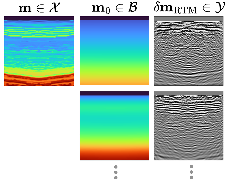
3.1 Jacobian-informed dataset with variability in \(\mathbf{m}_0\)
To ensure that the learned surrogate generalizes across different models, we construct a dataset that captures variability in both the groundtruth and background model. We draw pairs \((\mathbf{m}, \mathbf{m}_0) \sim \mu\) where \(\mathbf{m}_0\) is generated by applying randomized smoothing operations to the slowness field in either the depth or time domain (Figure 3). These perturbations introduce kinematic variability, resulting in shifts and distortions of migrated events (Figure 3). In addition to RTM images, \(\delta\mathbf{m}_{\mathrm{RTM}}\), we include action of Jacobian along a small set of informative directions shared across all models \(\bar{\mathbf{V}}_r = [\bar{\mathbf{v}}_1, ..., \bar{\mathbf{v}}_r]\), where \(r\) denotes the number of directions used. The resulting dataset is given by \[ \mathcal{D} = \left\{ \left( \mathbf{m}^{(i)}, \mathbf{m}_0^{(i)}, \delta \mathbf{m}_{\mathrm{RTM}}^{(i)}, \bar{\mathbf{V}}_r, \left(\frac{\partial \mathcal{R}}{\partial \mathbf{m}}\bigg|_{\mathbf{m}^{(i)}}\right)\bar{\mathbf{V}}_r \right) \right\}_{i=1}^{N} \] where \(i\) indexes training samples. This dataset enables training of a neural operator that is amortized across different groundtruth and background models, while learning accurate Jacobian along the directions that govern inversion updates.
3.2 Jacobian-informed training
With this training dataset, we train \(\mathcal{R}_{\mathrm{nn}}(\mathbf{m}, \mathbf{m}_0)\) to approximate the generalized RTM mapping as defined in Equation 1. In addition to matching the RTM images, we enforce accuracy in the learned Jacobian along the \(\bar{\mathbf{V}}_r\). This encourages the neural operator to learn sensitivities that are consistent with the physical inversion process. The training loss is: \[ \begin{aligned} \mathcal{L}_\text{train}(\mathbf{m}, \mathbf{m}_0) = &\|\mathcal{R}_{\mathrm{nn}}(\mathbf{m}, \mathbf{m}_0) - \delta \mathbf{m}_{\mathrm{RTM}}\|^2_2 \\ &+ \lambda \|\Bigl(\frac{\partial \mathcal{R}_{\mathrm{nn}}}{\partial \mathbf{m}} \Bigr) (\mathbf{m}, \mathbf{m}_0)\bar{\mathbf{V}}_r - \Bigl(\frac{ \partial \mathcal{R}}{ \partial \mathbf{m}} \Bigr) (\mathbf{m}, \mathbf{m}_0)\bar{\mathbf{V}}_r\|^2_2. \end{aligned} \] This regularization term encourages the surrogate to learn inversion-relevant sensitivities, leading to more accurate gradient directions during inversion.
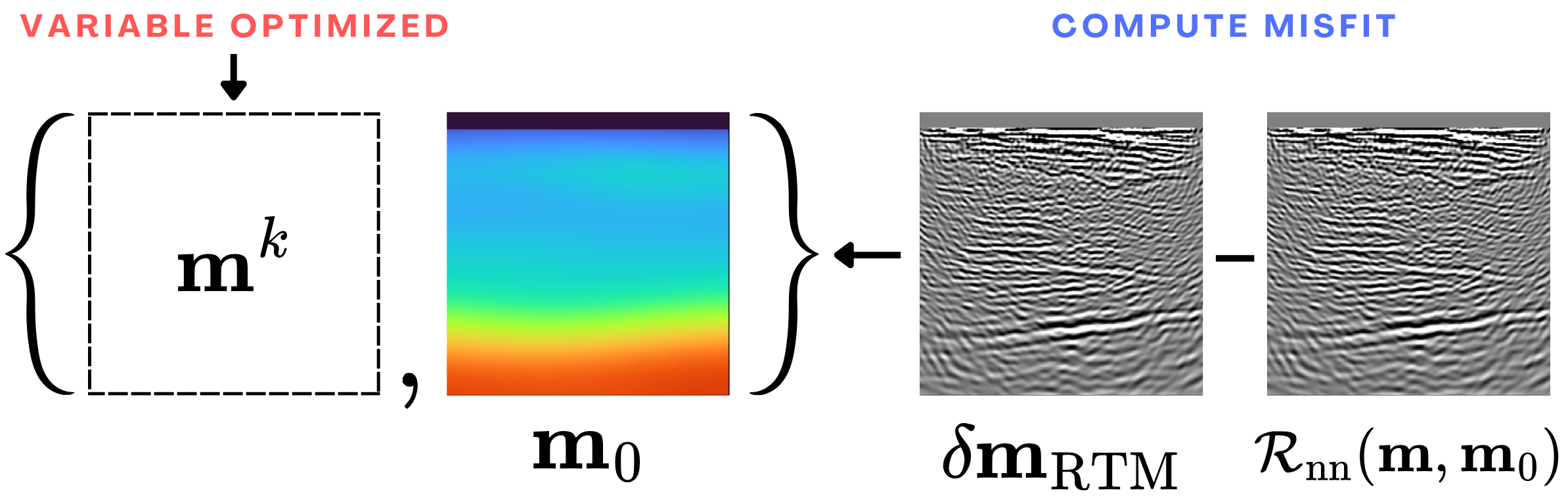
3.3 Least-Squares inversion with \(\mathcal{R}_{\mathrm{nn}}\)
After training, the neural surrogate, \(\mathcal{R}_{\mathrm{nn}}\), is used within a least-squares inversion framework. Given an observed RTM image \(\delta \mathbf{m}_{\mathrm{RTM}}\), we estimate the velocity model by solving \[\min_\mathbf{m} \|\mathcal{R}_{\mathrm{nn}}(\mathbf{m}, \mathbf{m}_0) - \delta \mathbf{m}_{\mathrm{RTM}}\|^2_2 \: \: \text{s.t.} \: \|\nabla \mathbf{m}\|_1 \leq \tau,\] where the total variation (TV) constraint promotes piecewise-smooth structure while preserving sharp interfaces and \(\tau\) controls the strength of the TV constraint (Esser et al. 2018; Peters and Herrmann 2017).
4 Numerical Experiments
We compare standard neural operators trained only with forward prediction loss against the proposed Jacobian-informed training.
4.1 Training Setup
To create the dataset, we use Julia package, JUDI.jl (Witte et al. 2019; Louboutin et al. 2023). Velocity models and RTM images are discretized to 256 x 256 (E. Jones et al. 2012). In this work, we use 202 training samples and 22 test samples.
We evaluate our training algorithm using FNO (Li et al. 2020), which models operators via global convolutions in Fourier space. We train two variants: (i) a standard FNO trained with forward loss, and (ii) a Jacobian-informed FNO (JI-FNO) with additional Jacobian supervision. To understand the impact of the number of directions in Jacobian we supervise, we train JI-FNO with 8 and 64 directions, which is 0.01% and 0.1% of the model of size, 256 x 256. Detailed schematic for training objective is shown in Figure 1.
4.2 Inversion setup
.png)
After training, \(\mathcal{R}_{\mathrm{nn}}\) replaces the physical operator within the inversion loop (Figure 2). For each test sample, inversion is performed by updating the velocity model while keeping the background model fixed (Ma and Alkhalifah 2025). The initial model is a smoothed version of the true velocity. Because the surrogate is differentiable, gradients can be computed efficiently via automatic differentiation, making each iteration significantly cheaper than wave-equation-based approaches. This allows us to run 1200 iterations of gradient-based optimization using Adam (Kingma and Ba 2014).
5 Result
| Metric | FNO | JI-FNO | JI-FNO |
|---|---|---|---|
| \(r\) | N.A. | 8 | 64 |
| Model Error (Rel. \(L_2\)) |
\(0.29\) | 0.21 | 0.21 |
| Data Residual (Rel. \(L_2\)) |
\(0.28\) | \(0.19\) | 0.12 |
| Recovered Model SSIM |
\(0.50\) | \(0.68\) | 0.76 |
Table 1 summarizes the inversion performance across all neural surrogates. Incorporating Jacobian supervision consistently improves both data fitting and model reconstruction quality. The JI-FNO reduces the relative model error by 8% and achieves significantly lower data residuals (decreases by 16%) compared to the standard FNO. In addition, structural similarity (SSIM) improves substantially (increases by 26%), indicating better recovery of subsurface features. These results show that aligning the surrogate with inversion-relevant sensitivities leads to more accurate gradient updates and improved convergence (as shown in Figure 6).
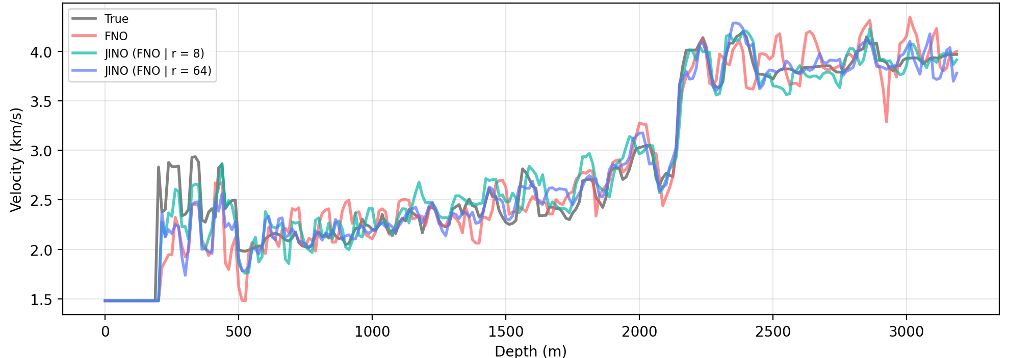
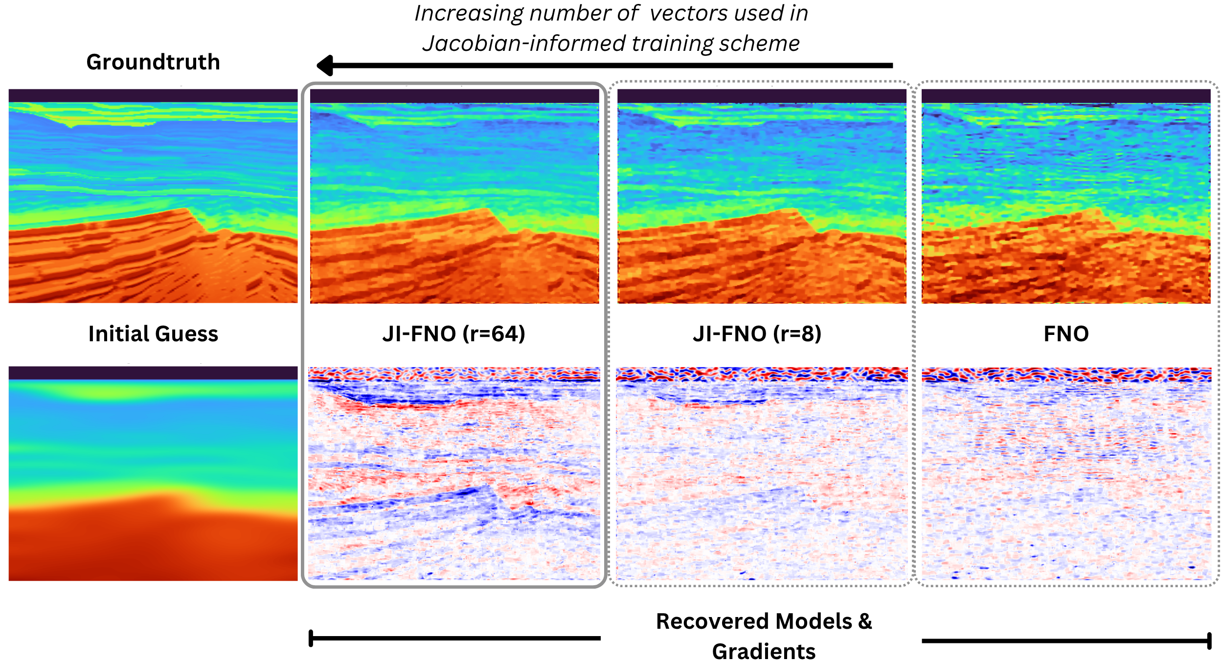
Figure 5 compares velocity models recovered using neural surrogates trained with different training strategies. The standard FNO (the right most column) produces reconstructions with noisy artifacts from mid to deep layers and exhibits distortions in the deeper high-velocity layers. In contrast, the Jacobian-informed models yield significantly cleaner images, with improved layer continuity and more accurate recovery at depth. Notably, even when using only 8 eigenvectors, the Jacobian-informed model already leads to substantial improvements over the baseline. Increasing the number of eigenvectors to 64 further enhances layer sharpness and continuity. These improvements are more pronounced in deeper regions (Figure 7).
We further analyze the gradients produced by each model (second row of Figure 5). Gradients from the standard FNO are dominated by high-frequency noise and lack coherent spatial structure. In contrast, the Jacobian-informed models produce gradients that are more structured and aligned with reflector geometry, particularly in the shallow to mid-depth regions. This difference explains the improved inversion performance: by learning gradients that follow the physically meaningful directions of the inverse problem, the proposed method produces more stable and accurate model updates.
6 Conclusion and discussion
We showed that accurate forward prediction alone is insufficient for surrogate-assisted seismic inversion, as inversion updates depend on the adjoint Jacobian. If a neural operator learns incorrect sensitivity, gradient-based updates may introduce unphysical artifacts and fail to recover deeper structures. By incorporating Jacobian supervision during training, the proposed approach ensures that the learned operator produces gradients consistent with the physical inversion geometry. Numerical experiments demonstrate that the proposed approach improves gradient quality, reduces artifacts, and yields more accurate recovery of deeper velocity structures compared to models trained with forward prediction loss alone. These results highlight that reliable surrogate modeling for seismic inversion requires learning inversion-relevant geometry, not just forward mappings.
Also, we observed as we add more directions during Jacobian-informed training, the surrogate Jacobian during inversion becomes increasingly accurate in model recovery. We therefore expect the benefits of the proposed approach to become even more pronounced in more challenging inversion scenarios, such as cases with poorer background models or limited training data, which we will continue to explore in the future work.
Lastly, the proposed approach has direct implications for Gauss–Newton FWI. Improving the accuracy of the learned Jacobian enables more accurate curvature information and search directions. This opens the possibility of using neural surrogates as data-driven nonlinear preconditioners, reducing the number of Gauss-Newton iterations while preserving inversion accuracy.
7 Acknowledgement
During the preparation of the work, the authors used ChatGPT to refine sentence structures of the manuscript. After using this service, the authors reviewed and edited the content as needed and take full responsibiltiy for the content of the publication.