SAGE: Subsurface AI-driven Geostatistical Extraction with proxy posterior
\[ \def\textsc#1{\dosc#1\csod} \def\dosc#1#2\csod{{\rm #1{\small #2}}} \]
Introduction
Characterization of subsurface physical properties (e.g., velocity, density, compressional wavespeed, impedence, Poisson ratio) is foundational to quantitative geoscience. These parameters govern wave propagation and provide key inputs to applications including resource exploration(Virieux and Operto 2009), reservoir monitoring (Gahlot, Orozco, et al. 2024; Gahlot, Li, et al. 2024), and prediction of subsurface fluid flow and storage (Park et al. 2026; Deng et al. 2025). In particular, within seismic exploration workflows, accurate velocity models are indispensable for both imaging and inversion, as they directly regulate the kinematics and recorded wavefields consequently, the fidelity of subsurface reconstruction and property estimation. Traditionally, velocity estimation has been addressed via Full Waveform Inversion (FWI) (Tarantola 1984); however, its high-dimensional, nonlinear, and ill-posed nature renders the problem challenging in practice.
Recent advances in generative networks and machine learning offer a data-driven answer to this challenge by introducing training approaches that allow creation of scalable and high-performance algorithms for velocity model building. Various approaches have been developed that formulate the task as Bayesian posterior inference with uncertainty quantification (Zeng et al. 2025; Jia et al. 2025). Subsequent works incorporate physics-informed representations and summary statistics, such as reverse-time migration (RTM) (Erdinc et al. 2025; Taufik and Alkhalifah 2026) or common image gathers (Yin et al. 2024; Orozco et al. 2024), to improve conditioning. Other methods leverage explicitly trained networks as priors and perform inversion via sampling-based schemes coupled with the forward operator (Brandolin and Alkhalifah 2026; Hu et al. 2025). Despite these advances, all the approaches fundamentally rely on having access to large-scale, geologically realistic, high-resolution velocity models for training (Li et al. 2026), which are often prohibitively scarce.
Inspired by self-supervised learning literature (Tachella and Davies 2026) and approaches (Daras et al. 2023; Aali et al. 2025), we propose SAGE, a novel approach that circumvents the need for fully observed velocity models. SAGE learns a proxy posterior over velocity fields using only migrated images and occluded velocity models (well-log measurements). The key contributions of SAGE are: (1) learning a proxy posterior from paired incomplete velocity and migrated image supervision; (2) amortized synthesis of high-resolution velocity realizations conditioned solely on migrated at inference; (3) utilization as a data sample generator for training downstream, task-specific networks; and (4) efficient fine-tuning on field migrated image and well-log data.
Theory and Methodology
Seismic imaging and Bayesian inference
The estimation of subsurface properties, such as the acoustic wavespeed field \(\mathbf{x}\), can be formulated as an inverse problem from recorded seismic data \(\mathbf{d}\). The relationship between the model parameters and the observed data is governed by the seismic wave equation through a nonlinear forward modeling operator: \(\mathbf{d} =\mathcal{F}(\mathbf{x}) + \boldsymbol{\epsilon},\boldsymbol{\epsilon} \sim p(\boldsymbol{\epsilon})\) where \(\mathcal{F}\) denotes the nonlinear forward operator mapping subsurface parameters to predicted wavefield measurements at receiver locations, and \(\boldsymbol{\epsilon}\) represents band-limited acquisition noise. Recovering the subsurface model \(\mathbf{x}\) from \(\mathbf{d}\) is challenging due to the strong nonlinearity of the forward operator, the presence of a nontrivial null space, and the compounding effects of noise and modeling errors. To mitigate these difficulties, we employ summary statistics (Orozco et al. 2023) that preserve key salient structural information while transforming the data into a more interpretable representation. In seismic imaging, a commonly used summary statistic is the reverse-time migration (RTM) image. Let \(\mathbf{x}_0\) denote a background model and let \(\mathbf{J}(\mathbf{x}_0) = \left.\frac{\partial \mathcal{F}}{\partial \mathbf{x}}\right|_{\mathbf{x}_0}\) denote the Jacobian of the forward operator evaluated at \(\mathbf{x}_0\). The RTM image is given by: \(\mathbf{y}=\mathbf{J}(\mathbf{x}_0)^ \top\left(\mathcal{F}(\mathbf{x}_0) - \mathbf{d}\right)\). Despite this transformation, the inverse problem remains ill-posed: multiple velocity model, \(\mathbf{x}\), can explain the observations equally well. This ambiguity motivates a probabilistic formulation. Within a Bayesian framework, the posterior distribution over model parameters is given by by Bayes’ rule: \(p(\mathbf{x} \mid \mathbf{y}) = \frac{p(\mathbf{y} \mid \mathbf{x}) p(\mathbf{x})}{p(\mathbf{y})},\) where \(p(\mathbf{x})\) denotes the prior distribution describing information about the velocity model before observing the data, and \(p(\mathbf{y} \mid \mathbf{x})\) is the likelihood, which measures how probable the observed RTM image \(\mathbf{y}\) is for a given model \(\mathbf{x}\). Classical Bayesian inference relies on evaluating the likelihood and prior to generate posterior samples. In this work, we instead estimate a proxy posterior \(\tilde{p}(\mathbf{x}|\mathbf{y})\) under the assumption that only occluded (partially observed) measurements of prior samples are available.
Simulation-based inference with conditional score-based networks
Simulation-based inference (SBI) is a framework that allows the training of surrogates for posterior using neural estimators (Cranmer, Brehmer, and Louppe 2020). The key idea is to use numerical simulators to generate training pairs \(\mathcal{D} = \{ (\mathbf{x}^{(i)}, \mathbf{y}^{(i)}) \}_{i=1}^{N}\), where each pair consists of a set of subsurface velocity \(\mathbf{x}^{(i)}\) and the corresponding observation \(\mathbf{y}^{(i)}\) derived using the forward simulation and linearized imaging. The resulting pairs \((\mathbf{x}^{(i)}, \mathbf{y}^{(i)})\) are then used to train a conditional generative network, which learns the posterior distribution of the velocities conditioned on migrated images. In this study, we will use conditional score-based generative networks in an SBI setting (Arruda et al. 2025).
Score-based diffusion networks are density estimators that learn the score function of a sequence of noise-perturbed distributions. Specifically, the network learns \(\nabla_{\mathbf{x}_t} \log p_t(\mathbf{x}_t)\) where \(p_t(\mathbf{x}_t)\) denotes the distribution of the data after corruption with Gaussian noise. In the variance-exploding formulation used in this work, the perturbed distribution can be written as \(p_t(\mathbf{x}_t) = p(\mathbf{x}) * \mathcal{N}(0, \sigma(t)^2 \mathbf{I})\) where \(t \in [0,1]\) denotes diffusion time and \(\sigma(t)\) is a monotonically increasing noise schedule. This construction corresponds to progressively perturbing samples from the data distribution with Gaussian noise of increasing variance, thereby inducing a continuum of distributions that interpolate between the data (\(\mathbf{x}\)) and an isotropic Gaussian. The forward diffusion process that generates these perturbed samples is governed by a stochastic differential equation (Song et al. 2020). This process induces a monotonic increase in variance, progressively perturbing samples until the distribution approaches an isotropic Gaussian. Once the score function \(\nabla_{\mathbf{x}_t} \log p_t(\mathbf{x}_t)\) has been learned, samples from the data distribution can be generated by simulating a reverse-time stochastic differential equation (Song et al. 2020). As proposed by (Karras et al. 2022), we adopt a simplified score-learning objective with \(\sigma(t) = t\). The training objective is given by: \[ \hat{\boldsymbol{\theta}} = \arg\min_{\boldsymbol{\theta}} \mathbb{E}_{\mathbf{x} \sim p(\mathbf{x})} \mathbb{E}_{\sigma \sim \mathrm{LogNormal}(P_{\mathrm{mean}}, P_{\mathrm{std}}^2)} \mathbb{E}_{\mathbf{n} \sim \mathcal{N}(0, \mathbf{I})} \left\| D_{\boldsymbol{\theta}}(\mathbf{x} + \sigma \mathbf{n}, \sigma) - \mathbf{x} \right\|_2^2, \] where the denoising network \(D_{\boldsymbol{\theta}}(\mathbf{x}_t, \sigma)\), with learnable parameters \(\boldsymbol{\theta}\), is trained to recover the clean signal \(\mathbf{x}\) from its noisy counterpart \(\mathbf{x}_t = \mathbf{x} + \sigma \mathbf{n}\), where \(\mathbf{n} \sim \mathcal{N}(0, \mathbf{I})\). The parameters \(P_{\mathrm{mean}}\) and \(P_{\mathrm{std}}\) define the \(\mathrm{LogNormal}\) distribution governing the noise levels \(\sigma\). The score function of the perturbed distribution can then be approximated as \(\nabla_{\mathbf{x}_t} \log p_t(\mathbf{x}_t) \approx \frac{D_{\boldsymbol{\theta}}(\mathbf{x}_t, \sigma) - \mathbf{x}_t}{\sigma^2}\). This formulation corresponds to the unconditional setting. To model conditional distributions, we extend the framework to estimate the conditional score \(\nabla_{\mathbf{x}_t} \log p_t(\mathbf{x}_t \mid \mathbf{y})\) where \(\mathbf{y}\) denotes the conditioning variable (e.g., migrated images). The corresponding training objective is modified to incorporate conditioning as follows: \[ \hat{\boldsymbol{\theta}} = \arg\min_{\boldsymbol{\theta}} \mathbb{E}_{(\mathbf{x},\mathbf{y},\sigma,\mathbf{n}) \sim p(\mathbf{x},\mathbf{y},\sigma,\mathbf{n})} \left\| D_{\boldsymbol{\theta}}(\mathbf{x} + \sigma \mathbf{n}, \mathbf{y}, \sigma) - \mathbf{x} \right\|_2^2. \] However, SBI approaches for posterior estimation typically require access to samples from the prior distribution \(p(\mathbf{x})\). In the proposed SAGE framework, we relax this requirement by learning from partially observed realizations of \(\mathbf{x}\) (velocities).
SAGE Framework

SAGE training
Input: \(D_{\boldsymbol{\theta}}\), \(p(\mathbf{x}_{\mathrm{obs}}, \mathbf{A}, \mathbf{y})\), \(p(\widetilde{\mathbf{A}} \mid \mathbf{A})\)
Repeat:
Sample \((\mathbf{x}_{\mathrm{obs}}, \mathbf{A}, \mathbf{y}) \sim p(\mathbf{x}_{\mathrm{obs}}, \mathbf{A}, \mathbf{y})\), \(\widetilde{\mathbf{A}} \sim p(\widetilde{\mathbf{A}} \mid \mathbf{A})\)
Set \(\widetilde{\mathbf{x}}_{\mathrm{obs}} \gets \widetilde{\mathbf{A}} \mathbf{x}_{\mathrm{obs}}\)
Sample \(\sigma \sim \operatorname{LogNormal}\), \(\mathbf{n} \sim \mathcal{N}(\mathbf{0}, \mathbf{I})\)
Set \(\widehat{\mathbf{x}} \gets D_{\boldsymbol{\theta}}(\widetilde{\mathbf{x}}_{\mathrm{obs}} + \sigma \mathbf{n}, \mathbf{y}, \widetilde{\mathbf{A}}, \sigma)\)
Update \(\boldsymbol{\theta} \gets \boldsymbol{\theta} - \eta \nabla_{\boldsymbol{\theta}} \|\mathbf{A}\widehat{\mathbf{x}} - \mathbf{x}_{\mathrm{obs}}\|_2^2\)
Until convergence
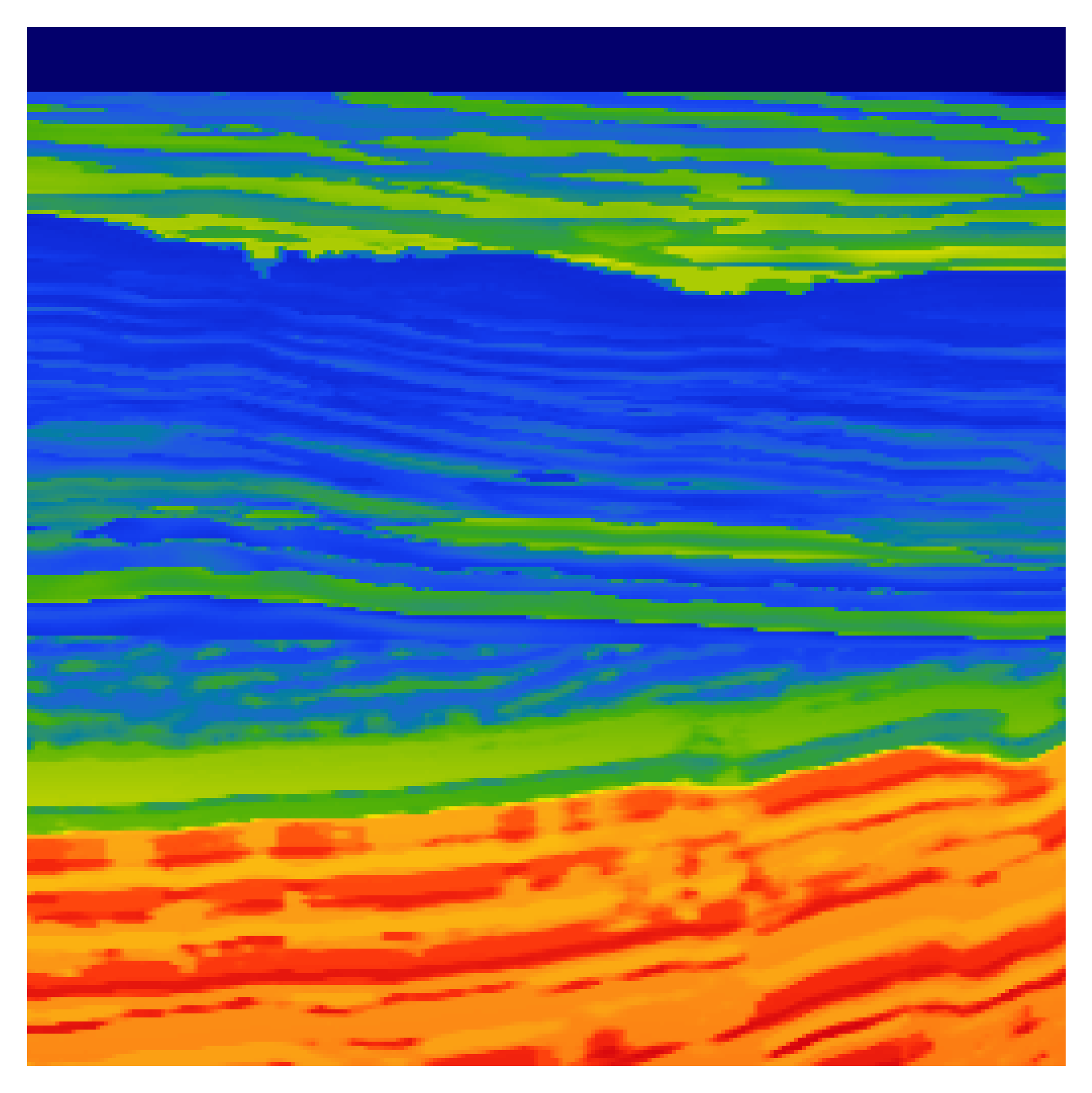
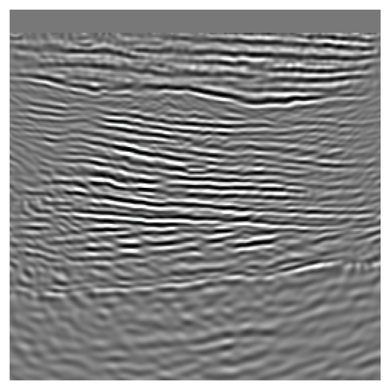
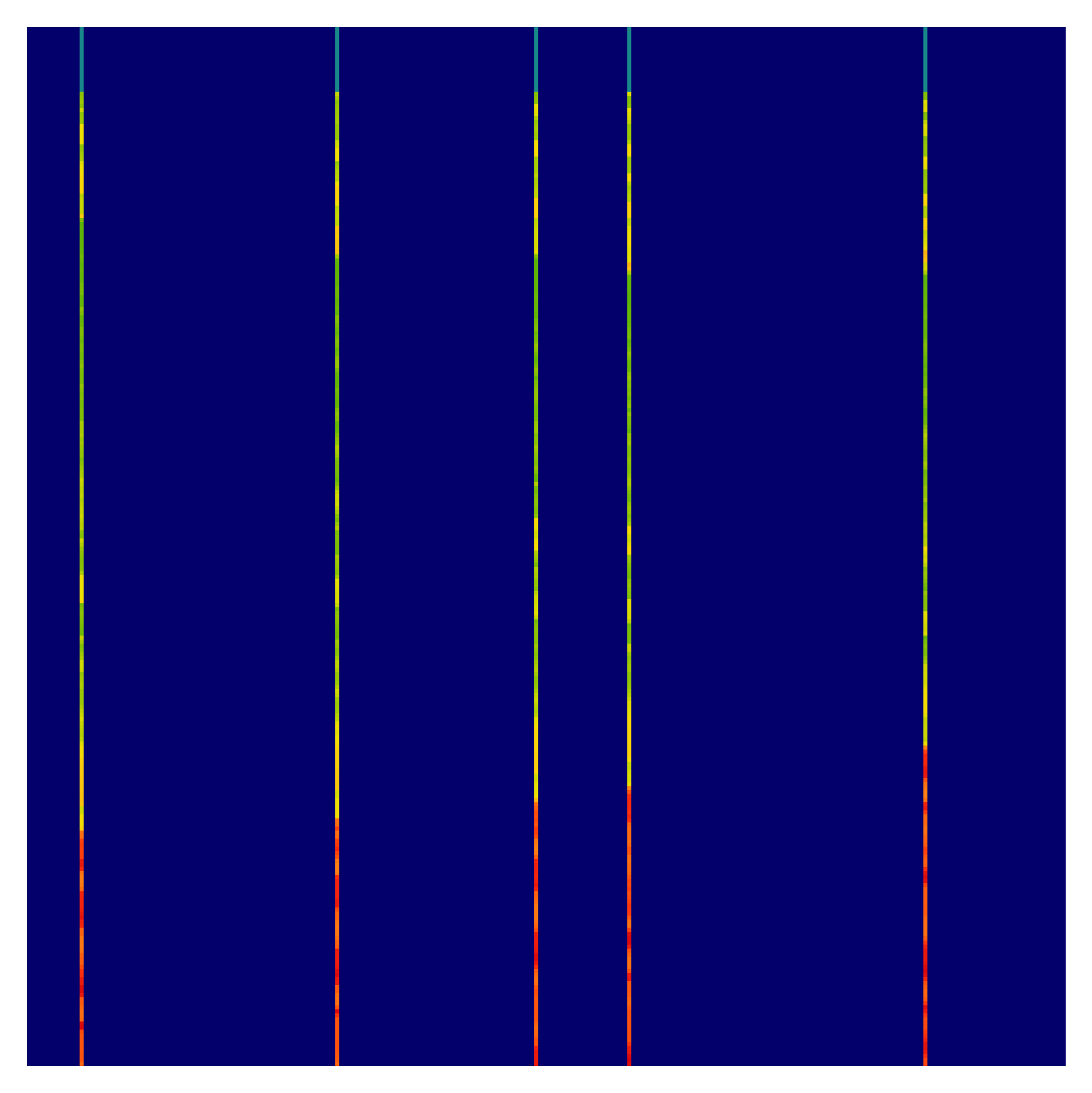
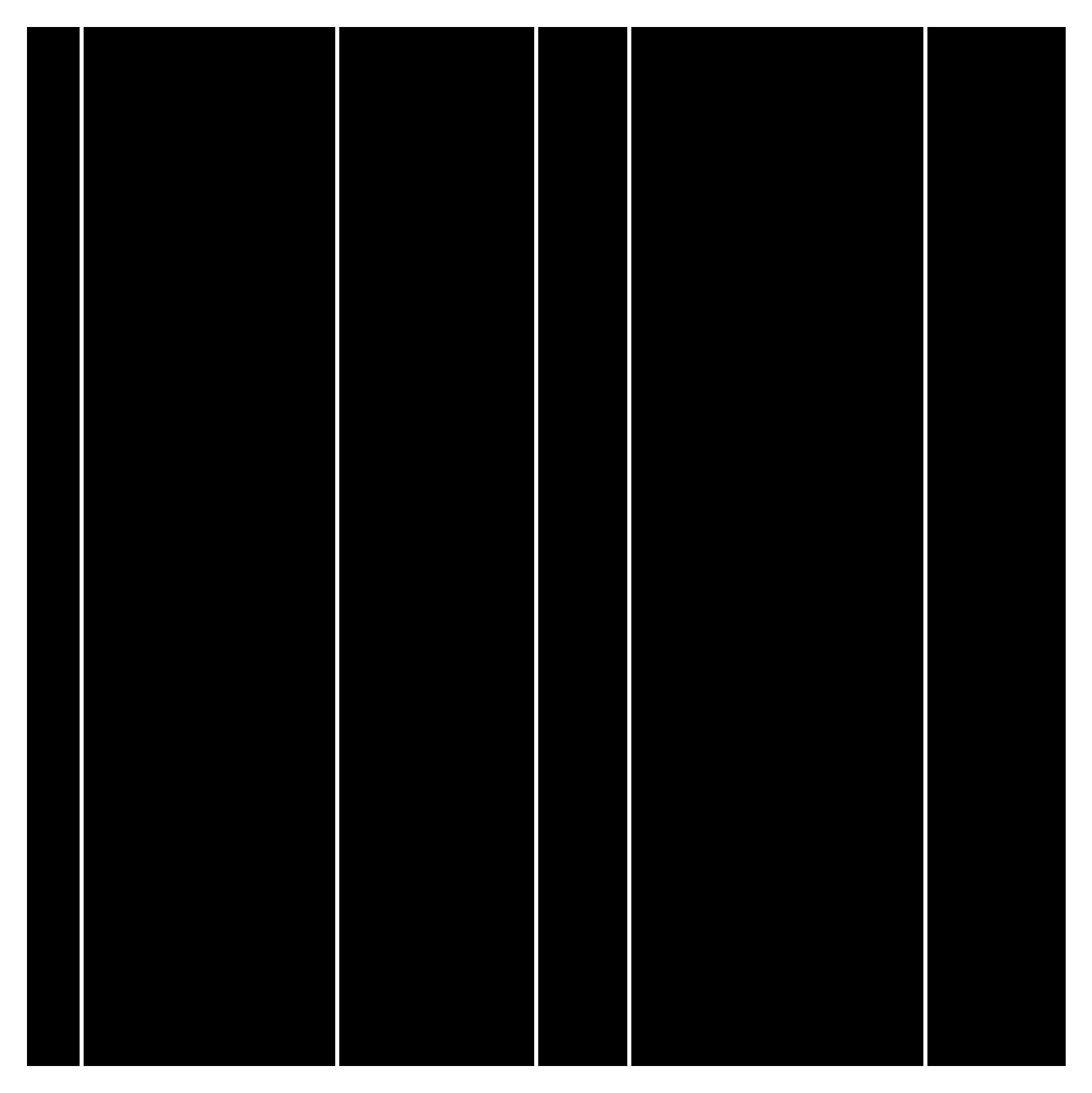
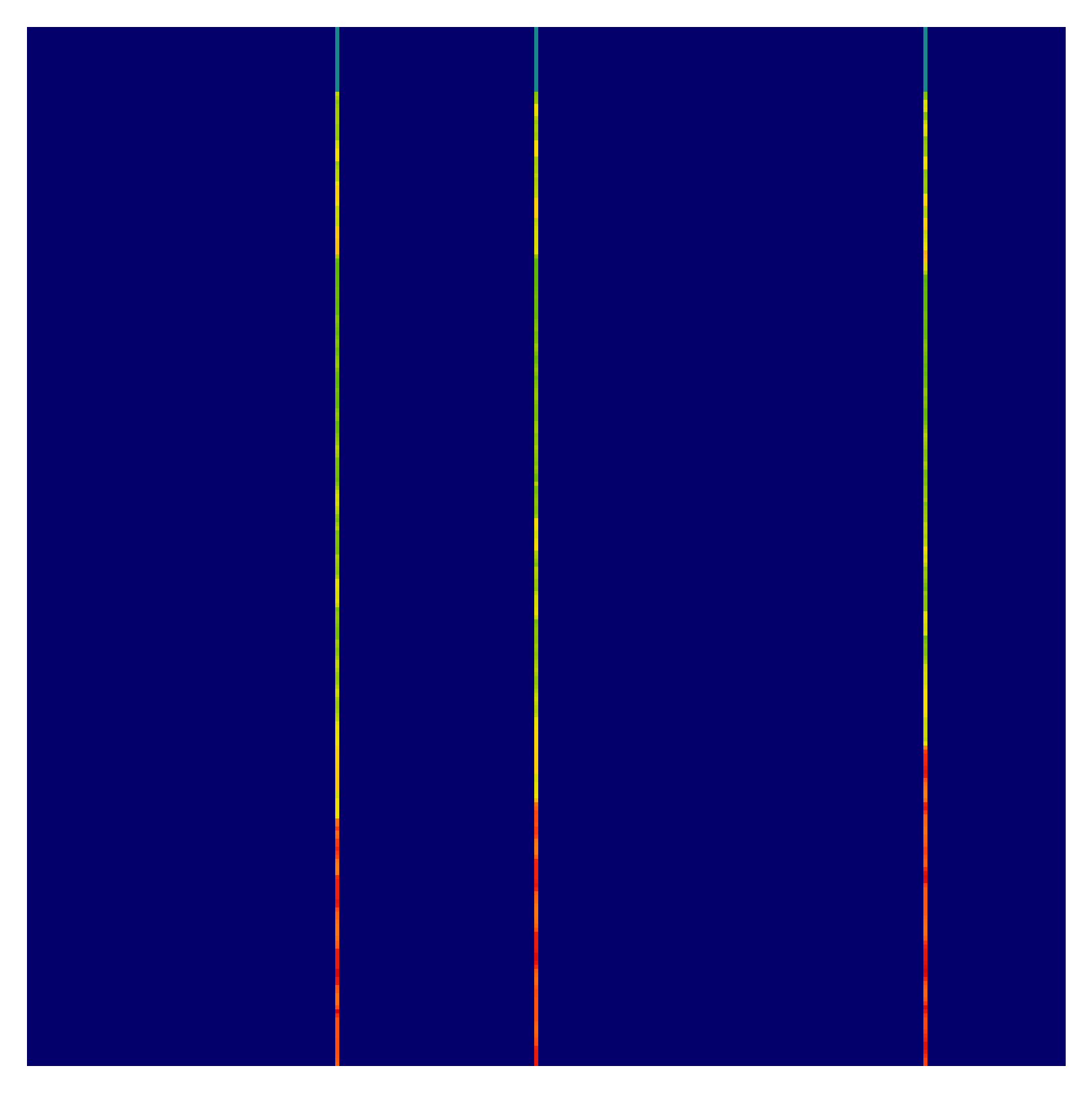
We consider a setting in which direct access to prior velocity samples \(\mathbf{x} \sim p(\mathbf{x})\), with \(x \in \mathbb{R}^N\) where \(N=n_x \times n_z\) is unavailable. Instead, we observe only sparse, but direct, measurements of the velocity field obtained from well logs denoted by \(\mathbf{x}_\text{obs}\) together with corresponding seismic summary statistics \(\mathbf{y}\) derived from RTM. Well-log measurements correspond to column-wise observations of the velocity field and can be represented as a masking operation. Let \(\mathbf{w} \in \{0,1\}^{n_{x}}\) vector specifying which lateral positions are observed. This induces a masking operator \(\mathbf{A} \in \mathbb{R}^{N \times N}\) acting on unseen \(\mathbf{x}\) defined as \(A = \{\text{diag}(\mathbf{w} \otimes \mathbf{1}_{n_{z}}): \mathbf{w} \in \{0,1\}^{n_{x}}\}\), where \(\otimes\) denotes the Kronecker product, \(\mathbf{1}_{n_z} \in \mathbb{R}^{n_z}\) is a vector of ones and the operator \(\mathrm{diag}(\cdot)\) maps a vector to a diagonal matrix with that vector on its diagonal. The observed velocity measurements are then given by \(\mathbf{x}_\text{obs} = \mathbf{A}\mathbf{x}\). In practice, well locations vary across surveys; we model this variability by treating the indicator vector as a random variable \(\mathbf{w} \sim p(\mathbf{w})\), which in turn induces a stochastic \(\mathbf{A} \sim p(\mathbf{A})\). Since only incomplete observations of \(\mathbf{x}\) are available, direct characterization of the posterior distribution \(p(\mathbf{x} \mid \mathbf{y})\) is intractable. This limitation motivates the introduction of a proxy posterior distribution \(\tilde{p}(\mathbf{x} \mid \mathbf{y})\) that can be learned from jointly available RTM images and partial well-log measurements. Taking note from the previous section, posterior estimation can be recast within the denoising formulation of score-based networks. A naïve approach is to enforce consistency of the denoiser with observed velocity measurements through the measurement operator. This leads to the following objective: \[ \hat{\boldsymbol{\theta}} = \arg\min_{\boldsymbol{\theta}} \mathbb{E}_{(\mathbf{y}, \mathbf{x}_{\mathrm{obs}}, \sigma, \mathbf{n}, \mathbf{A})} \left\| \mathbf{A}\, D_{\boldsymbol{\theta}}(\mathbf{x}_{\mathrm{obs}} + \sigma \mathbf{n}, \mathbf{y}, \mathbf{A}, \sigma) - \mathbf{x}_{\mathrm{obs}} \right\|_2^2, \] where \(\mathbf{n} \sim \mathcal{N}(0, \mathbf{I})\) and \(\mathbf{A} \sim p(\mathbf{A})\). However, this formulation admits a trivial solution given by \(D_{\boldsymbol{\theta}}(\cdot) = \mathbf{A}^\dagger \mathbf{x}_{\mathrm{obs}}\), where \(\mathbf{A}^\dagger\) denotes pseudo-inverse of \(\mathbf{A}\). This solution is undesirable, as it merely reconstructs the velocity field at observed locations while leaving unobserved regions unconstrained and effectively disregarding the conditioning information provided by the RTM image \(\mathbf{y}\). To prevent convergence to the trivial solution, we introduce a secondary masking (subsampling) operator that acts as a stochastic submask of the original masking operator. We define subsampling mask (Erdinc, Orozco, and Herrmann 2024): \[ \widetilde{\mathbf{A}} = \{\text{diag}(\tilde{\mathbf{w}} \otimes \mathbf{1}_{n_{z}}): \tilde{\mathbf{w}} \in \{0,1\}^{n_{x}}\} \ \text{with} \ \tilde{\mathbf{w}_i} \leq \mathbf{w}_i \ \forall \text{i = 1}, \ldots, n_{x} \] where \(\tilde{\mathbf{w}}\) is a binary vector that selects a subset of the originally observed columns. By construction, \(\widetilde{\mathbf{A}}\) cannot reveal previously unobserved entries and therefore constitutes a random submask of \(\mathbf{A}\). Applying this operator yields a further subsampled observation as \(\tilde{\mathbf{x}}_\text{obs} = \widetilde{\mathbf{A}}\mathbf{x}_\text{obs} = \widetilde{\mathbf{A}} \mathbf{A}\mathbf{x} = \widetilde{\mathbf{A}}\mathbf{x}\) where the last equality follows from the diagonal structure of the masking operators. We model this process as \(\widetilde{\mathbf{A}} \sim p(\widetilde{\mathbf{A}}| \mathbf{A})\) and \(\tilde{\mathbf{x}}_\text{obs} = \widetilde{\mathbf{A}}\mathbf{x}\). Using these subsampled observations, we define a training objective that enforces global reconstruction while maintaining consistency with the original measurements: \[ \hat{\boldsymbol{\theta}} = \arg\min_{\boldsymbol{\theta}} \mathbb{E}_{p_{\mathrm{train}}} \left\| \mathbf{A}D_{\boldsymbol{\theta}}(\tilde{\mathbf{x}}_{\mathrm{obs}}+\sigma\mathbf{n},\mathbf{y},\widetilde{\mathbf{A}},\sigma) -\mathbf{x}_{\mathrm{obs}} \right\|_2^2 \] with \(p_{\mathrm{train}}=p(\mathbf{y},\mathbf{x}_{\mathrm{obs}},\tilde{\mathbf{x}}_{\mathrm{obs}},\sigma,\mathbf{n},\mathbf{A},\widetilde{\mathbf{A}})\). The training procedure is summarized in (alg-sage-training?), while the matrix representations of the observations and the diagonal of masking operators are illustrated in Figure 1.A key characteristic of SAGE is that it simultaneously performs generative modeling and inpainting, enabling the reconstruction of globally consistent velocity fields from partial observations. Once training is complete, posterior sampling is performed by initializing the unobserved components with noise and iteratively applying the learned denoising dynamics conditioned on the RTM image. This procedure yields samples from the learned proxy posterior distribution.
Result and Numerical Study
SAGE Inference on synthetic wells
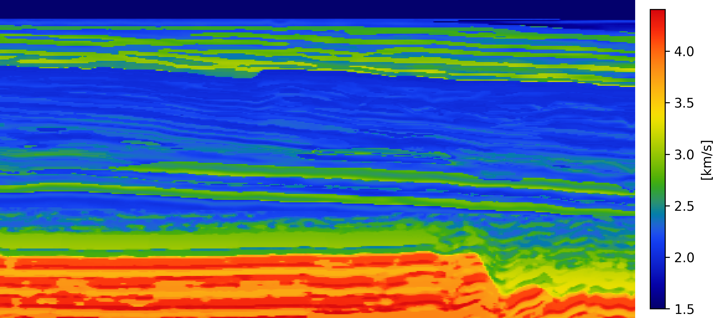
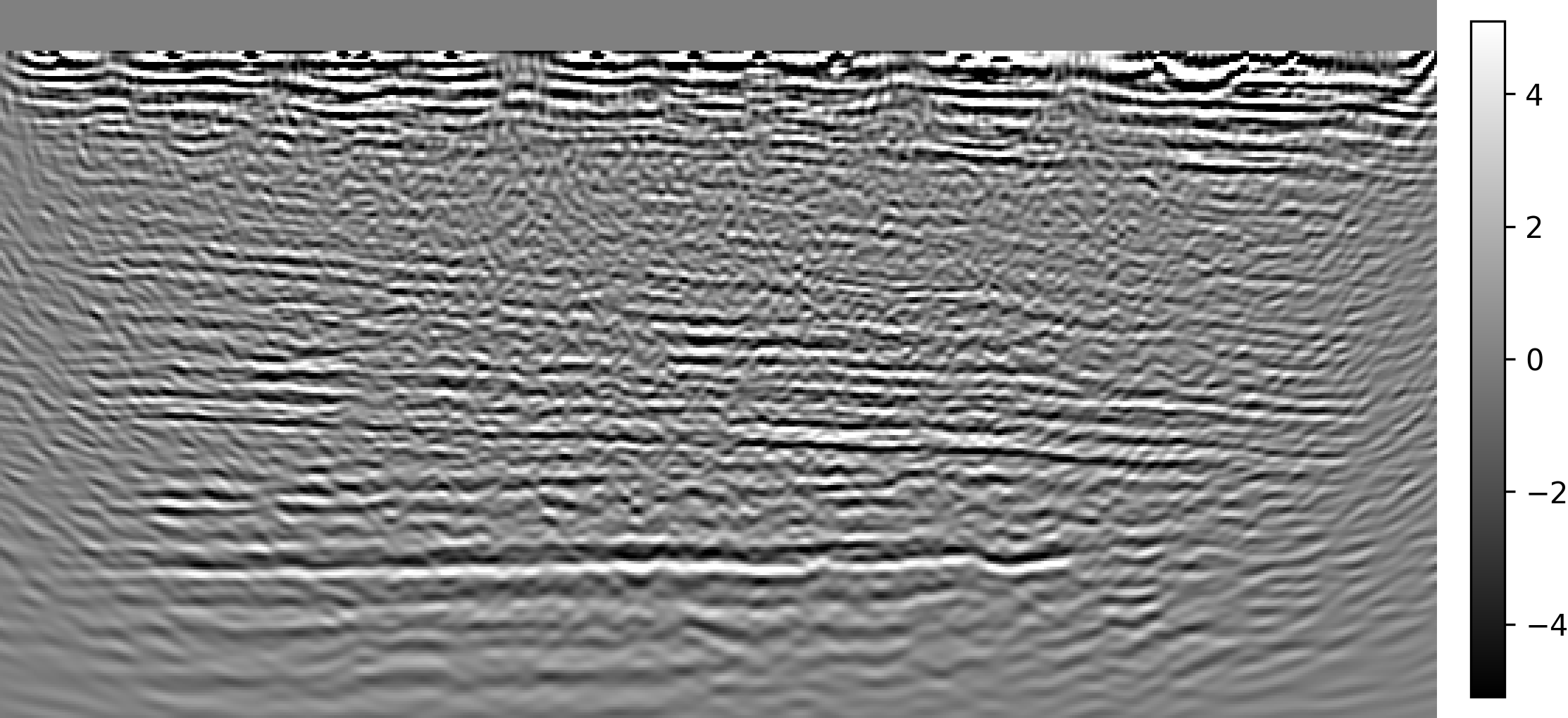
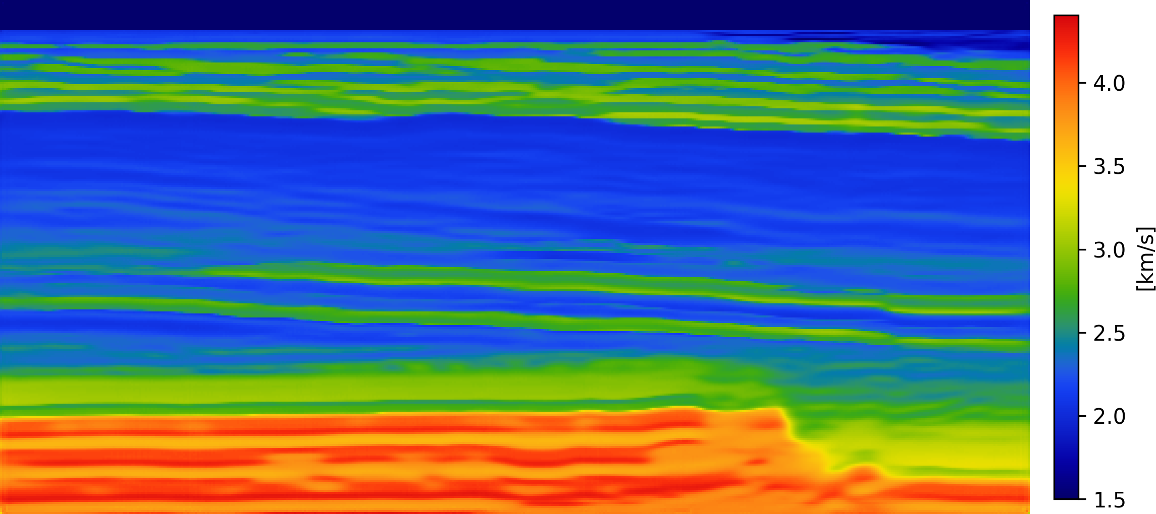
To evaluate SAGE, first we slice synthetic 2D Earth acoustic velocity models derived from the 3D Compass model, which is representative of geological formations in the North Sea region (E. Jones et al. 2012). The dataset consists of 1000 velocity realizations, each defined on a \(256\times 512\) grid with a spatial resolution of \(12.5\) meters, covering an area of \(3.2km\times 6.4\mathrm{km}\). Then for each velocity model, seismic data are simulated using \(16\) sources and \(256\) receivers, with Ricker wavelet centered at the dominant frequency of \(20\mathrm{Hz}\) and a recording duration of \(3.2\) seconds. To simulate realistic acquisition conditions, \(10\mathrm{dB}\) colored Gaussian noise is added to the shot records. RTM images are generated using a Gaussian-smoothed 2D background velocity model. Both wave simulation and migration are implemented using JUDI (Louboutin et al. 2023). This procedure yields a dataset of paired RTM images and corresponding full-resolution velocity models. However, in the SAGE setting, access to complete velocity models is not assumed. Therefore, we retain 5 out of 256 columns for each model and zero out the remaining entries, effectively removing approximately 99% of the information. These retained columns represent sparsely distributed well-log measurements that are spatially co-located (tied) with the RTM images.
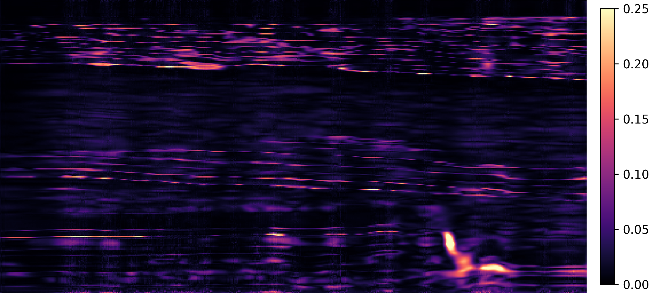
SAGE is trained using the procedure described in (alg-sage-training?). During training, the RTM image and corrupted subsampling mask are concatenated with the noisy, partially observed velocity field and provided as input to the network. A U-Net architecture is employed as the denoiser, and the total training time is approximately 20 GPU hours. For evaluation, we select unseen RTM examples withheld during training and generate samples from the learned proxy posterior using the trained network. Figure 2 presents the inference results obtained with SAGE. The posterior mean accurately reconstructs the dominant features of the ground-truth velocity model, achieving a structurally consistent estimate with an SSIM score of 0.82. The posterior standard deviation further provides a meaningful quantification of uncertainty, with elevated variance localized in regions characterized by increased geological complexity. We emphasize that, although comparisons are made against the ground truth for evaluation purposes, SAGE is trained exclusively on partially observed velocity fields and has no access to complete models during training. Consequently, mild smoothing of fine-scale structures is expected and reflects the inherent ambiguity induced by incomplete observations rather than a deficiency of the network.
Training of WISE with SAGE samples
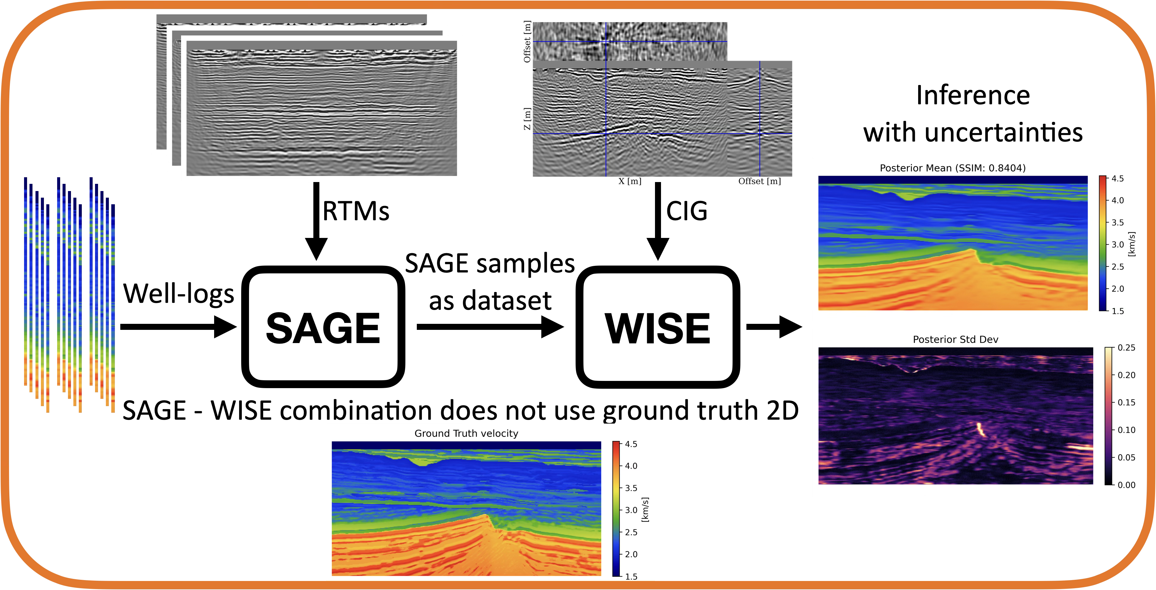
A prominent downstream application of SAGE is the generation of synthetic velocity samples for training specialized inversion networks. In this work, we consider WISE (Yin et al. 2024), a variational inference-based framework for FWI that produces ensembles of migration velocity models conditioned on common-image gathers (CIGs). The key advantage of WISE lies in its use of high-dimensional CIGs during inference, which provide stronger kinematic constraints than RTM images and are closer to a unitary mapping even under imperfect migration velocities (Hou and Symes 2016). Despite this advantage, WISE requires access to large collections of high-quality, fully observed velocity models during training, which limits its applicability in data-scarce settings. To address this limitation, we generate velocity samples from SAGE for unseen test examples and use these samples as a training dataset. The overall workflow is illustrated in Figure 3. Inference results indicate that WISE trained on SAGE samples yields high-quality velocity estimates, as reflected in both posterior mean and associated uncertainty maps. Notably, compared to training on ground-truth velocity models, the use of SAGE-generated samples incurs only a modest degradation in performance, with SSIM decreasing from 0.88 to 0.84.
SAGE inference on real seismic images and well data
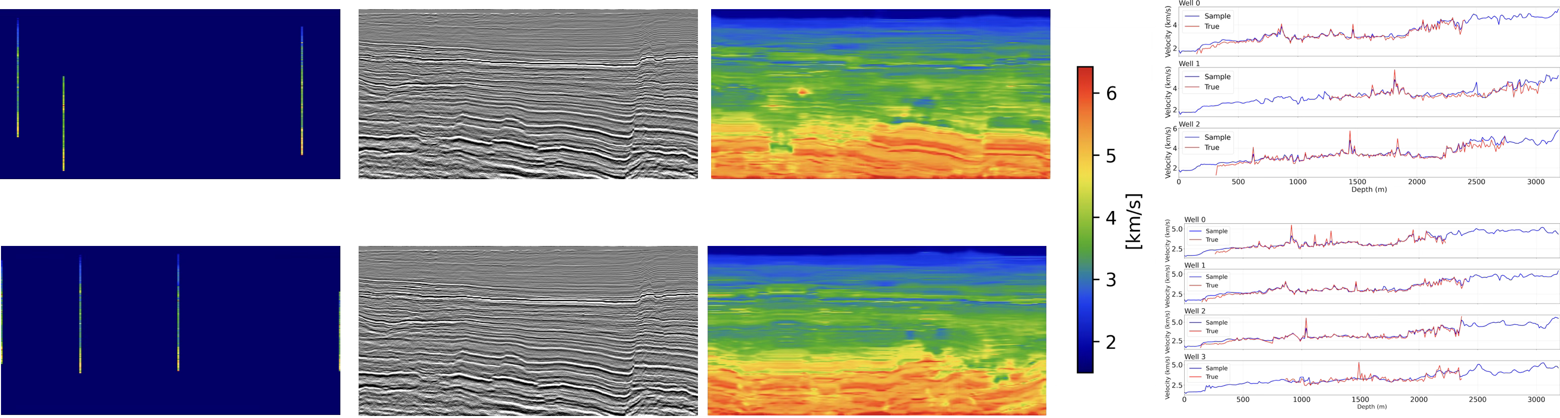
We evaluate the performance of SAGE on real seismic and well-log obtained from the UK National Data Repository (North Sea Transition Authority 2026). Following an preprocessing pipeline, including checkshot based time-to-depth conversion, well tie, quasi-2D line extraction, and kinematically consistent downsampling, we curate a dataset for training and evaluation. Additional details on the data preparation can be found in (Bhar et al. 2025). Due to the limited availability of well-log measurements (40 wells), we adopt a fine-tuning strategy in which a network pre-trained on the synthetic Compass model is adapted to the real data. Figure 4 presents the preliminary inference results of SAGE on real seismic data. The generated velocity models exhibit complex geological structure, aligning with the features observed in the migrated images while remaining consistent with independent well-log measurements not used during inference. We anticipate further improvements in performance as the training dataset is expanded.
Conclusion and Future Work
We introduced SAGE, a framework for subsurface velocity generation from incomplete observations, leveraging well-logs and migrated images. SAGE learns a proxy posterior during training and, at inference, produces full velocity fields conditioned solely on seismic migrated images, with well information implicitly encoded. Experiments demonstrate that SAGE produces high-quality and geologically consistent velocity models that can be utilized for downstream tasks, including training specialized learned inversion frameworks such as WISE. Notably, even with severely limited well-log data, fine-tuning on real seismic observations yields statistically plausible velocity realizations. Future work will extend SAGE to three-dimensional settings and larger curated field datasets.
Acknowledgement
This research was carried out with the support of Georgia Research Alliance, partners of the ML4Seismic Center. We acknowledge that we used data from UK National Data Repository and it contains information provided by the North Sea Transition Authority and/or other third parties. The authors used ChatGPT to refine sentence structures and improve readability. After using this service, the authors reviewed and edited the content as needed and take full responsibility.