Bridging the Acoustic-Elastic Gap in Seismic Inversion via Robust Summary Statistics
Simulation-based seismic inversion provides a principled framework for uncertainty quantification, but its performance degrades when the physics used in simulation differ from those of observed data. In practice, seismic inversion is often misspecified because the true physics are only partially known or too costly to model at scale, making field observations out of distribution relative to the simulations used for training; here, we study this issue through the acoustic-elastic gap. We introduce ElasNet, a misspecification-robust probabilistic inversion framework that bridges acoustic simulations and elastic observations through physics-informed summary statistics. We use acoustically imaged common-image gathers (CIGs) as structured summaries of seismic data, compress them with an attention-based summary network, and use maximum mean discrepancy (MMD) to align acoustic and elastic feature distributions during training while learning a conditional normalizing flow for posterior estimation with only acoustic data. Experiments on 2D Compass models show that the proposed approach reduces acoustic-elastic discrepancies in inferred velocity models and improves structural consistency and uncertainty calibration. These results demonstrate that robust summary statistics and distribution matching provide a scalable pathway for simulation-based seismic inversion under realistic physics mismatch.
\[ \def\textsc#1{\dosc#1\csod} \def\dosc#1#2\csod{{\rm #1{\small #2}}} \]
INTRODUCTION
Seismic inversion seeks to estimate subsurface seismic properties from recorded wavefields and forms the foundation of many geophysical applications, including reservoir characterization, subsurface hazard assessment, and time-laspe monitoring of subsurface changes (Tarantola 1984; Virieux and Operto 2009). The problem is inherently ill-posed and nonlinear because the relationship between subsurface parameters and recorded wavefields is highly complex, leading to non-uniqueness and sensitivity to noise and modeling assumptions.
To address these challenges and quantify uncertainty, recent work has increasingly adopted simulation-based inference (SBI) (Cranmer, Brehmer, and Louppe 2020; Orozco et al. 2023; Gahlot et al. 2025). Instead of producing a single deterministic estimate, SBI learns the posterior distribution of subsurface parameters conditioned on observations by leveraging large ensembles of synthetic simulations. This likelihood-free Bayesian framework bypasses the need to explicitly evaluate the likelihood function, whose repeated evaluation becomes computationally prohibitive when performing uncertainty quantification for high-dimensional seismic data governed by nonlinear wave physics (Orozco et al. 2023). As a result, SBI provides a promising pathway toward uncertainty-aware seismic inversion.
However, the reliability of SBI critically depends on the fidelity of the forward simulations used to generate the shot records as training data (Yin et al. 2024). In practice, simplified acoustic wave equations can be preferred for large-scale seismic simulations due to the high computational cost of repeated elastic forward modeling. In contrast, real seismic data are generated by elastic wave propagation in the Earth that includes both P- and S-wave phenomena and can change the reflection response at interfaces such as the ocean bottom or top salt (Virieux and Operto 2009). This discrepancy introduces model misspecification: the training simulations do not follow the same physics as the observed data. Consequently, models trained purely on acoustic simulations can produce biased posterior estimates and poorly calibrated uncertainty when applied to elastic observations (Farris, Clapp, and Araya-Polo 2023; Kelly et al. 2025). Although training directly on elastic simulations or field data would reduce this mismatch, elastic modeling is much more computationally expensive than acoustic modeling and acquired field data are limited(Farris, Clapp, and Araya-Polo 2023; Araya-Polo, Farris, and Florez 2019). There is therefore a growing need for approaches that can cope with simulation misspecification, enabling machine-learning models to learn from abundant simulated data while being adapted using a limited number of unpaired observations from the target domain. Here, we investigate this through the acoustic–elastic gap, using acoustic simulations as the abundant training data and elastic data as a proxy for field observations.
A key challenge in addressing this simulation–reality gap is the high dimensionality of raw seismic data which consist of time samples recorded over many sources and receivers. Directly conditioning learning algorithms on such shot records can be computationally demanding and vulnerable to modeling mismatch (Siahkoohi et al. 2023). Instead, physics-informed summary statistics can provide a more structured representation of the data (Orozco et al. 2023). In seismic imaging, common-image gathers (CIGs) are obtained by applying the adjoint of the (extended) Born modeling operator, mapping recorded data to the subsurface domain. This process removes much of the wave-propagation complexity while preserving offset-dependent focusing information that is strongly linked to velocity errors . Thus, CIGs provide a more stable and interpretable feature space for learning-based inversion than raw waveforms. Most importantly, they preserve offset-dependent information even when the background velocity model is inaccurate.
In this work, we introduce ElasNet, a probabilistic framework that bridges acoustic simulations and elastic observations through robust summary representations. Our approach maps seismic data to CIGs and compresses these features using an attention-based summary network that extracts informative offset-dependent patterns. To mitigate acoustic–elastic model misspecification, we align the feature distributions of acoustic CIGs generated from acoustic simulations and elastic CIGs obtained by acoustically imaging elastic data using maximum mean discrepancy (MMD) (Gretton et al. 2012) while training a conditional normalizing flow to estimate the posterior distribution of velocity models. This strategy enables posterior learning from inexpensive acoustic simulations while using MMD to align their summary features with those from a limited set of unpaired elastic data during training.
Through synthetic experiments on the Compass dataset (Jones et al. 2012), we demonstrate that ElasNet reduces discrepancies between acoustic and elastic posteriors, mitigates the spurious contrast at the ocean bottom, and improves structural consistency of inferred velocity models. These results suggest that combining physics-informed summaries with distribution alignment potentially offers a practical pathway for simulation-based seismic inversion under realistic physics mismatch.
METHODOLOGY
In the acoustic case, the modeled wavefield is the scalar pressure field \(p(t,\mathbf{r})\), with simulated data \(\mathbf{y}_{\mathrm{ac}}=\mathcal{F}_{\mathrm{ac}}(\mathbf{x})\), where \(\mathcal{F}_{\mathrm{ac}}\) denotes the variable-density isotropic acoustic wave-equation solution operator restricted to the receivers. In the elastic case, the modeled state is multicomponent and the recorded observable is the particle-velocity field \(\mathbf{v}(t,\mathbf{r})\), with simulated data \(\mathbf{y}_{\mathrm{el}}=\mathcal{F}_{\mathrm{el}}(\mathbf{x})\), where \(\mathcal{F}_{\mathrm{el}}\) denotes the isotropic first-order velocity–stress operator. Because pressure and particle velocity differ by a time derivative in the wave-equation formulation, the acoustic and elastic simulations correspond to different measurements.
To account for the difference between pressure measurements \(p(t,\mathbf{r})\) and particle-velocity measurements \(\mathbf{v}(t,\mathbf{r})\), we adopt a source convention that reflects the corresponding time-derivative relationship between these shot records. Specifically, we modify the acoustic source term by applying a time integral \(\mathbf{q}_{\mathrm{ac}}(t)\mapsto \partial_t^{-1}\mathbf{q}_{\mathrm{ac}}(t)\), thereby compensating for the different observables used in the acoustic and elastic wave-equation formulations.
Directly conditioning posterior estimation on raw shot records is computationally expensive and sensitive to acquisition- and physics-related mismatch. One way to reduce the dimensionality of seismic data is reverse-time migration (RTM), which applies the adjoint of the linearized Born modeling operator to map information from the data domain to the image domain (Biondi and Tisserant 2004). However, RTM-based summaries can be sensitive to inaccuracies in the background velocity model. To obtain a more informative and structured representation, we instead use subsurface-offset common-image gathers (CIGs) as physics-informed summary statistics (Geng et al. 2022; Orozco et al. 2023; Yin et al. 2024). CIGs are formed through the adjoint of the extended Born modeling operator, which maps the recorded wavefield into the subsurface domain while preserving offset-dependent focusing information and providing a summary that remains informative for posterior estimation even when the background velocity model is imperfect. For a fixed background velocity model \(\mathbf{x}_0\), CIGs are constructed as
\[\begin{equation} \bar{\mathbf{y}}(\mathbf{x}_0,\mathbf{y}) = \overline{\nabla \mathcal{F}}(\mathbf{x}_0)^\top \mathbf{y}, \end{equation}\]
where \(\mathbf{y}\) denotes the recorded wavefield data or the corresponding residual relative to data from \(\mathbf{x}_0\).
Attention-based summary representation
Although CIGs provide a physics-informed reduced representation of the seismic data, they remain high-dimensional because each spatial location is associated with a horizontal subsurface offset axis. To obtain a compact representation suitable for posterior estimation and distribution alignment, we introduce a learned summary network \(h_{\psi}(\cdot)\) that compresses the CIG while preserving informative offset-dependent information.
Given a CIG \(\bar{\mathbf{y}} \in \mathbb{R}^{m_x \times m_z \times m_h}\), where \(m_x,m_z\) denote the spatial dimensions of the velocity model and \(m_h=51\) denotes the offset-channel dimension, we treat the offset responses at each spatial location as a token. Treating the offset response at each spatial location as a token, the summary network applies self-attention within local \(8 \times 8\) spatial windows so that each location can aggregate nearby offset-dependent information and suppress less informative features. In our implementation, queries are formed from the token embeddings, while keys and values are computed from the collection of CIG tokens, enabling the network to emphasize coherent focusing patterns and suppress less informative responses.
The resulting attention features are projected through a \(1\times1\) convolution to reduce the channel dimension to a compact latent representation with \(d_c \in [6,10]\) channels. The output \(h_{\psi}(\mathbf{Y})\) therefore provides a compressed embedding of the CIG suitable for posterior velocity models estimation and distribution matching. This summary construction performs two levels of dimension reduction: a physics-informed reduction from shot records to CIGs, followed by a learned reduction from CIGs to compact latent features.
Maximum mean discrepancy
After mapping acoustic and elastic CIGs to compact summary representations through \(h_{\psi}\), we align their feature distributions using maximum mean discrepancy (MMD) (Gretton et al. 2012), a kernel-based distance widely used for two-sample testing and distribution matching.
Let \(p\) and \(q\) denote two distributions over a space \(\mathcal{Y}\) and let \(k(\cdot,\cdot)\) be a positive-definite kernel. The squared MMD between \(p\) and \(q\) is defined as \[\begin{align} \mathrm{MMD}^2(p, q) &= \mathbb{E}_{y,y' \sim p} [ k(y, y') ] \notag \\ &\quad + \mathbb{E}_{\tilde{y},\tilde{y}' \sim q} [ k(\tilde{y}, \tilde{y}') ] \notag \\ &\quad - 2\, \mathbb{E}_{y \sim p,\, \tilde{y} \sim q} [ k(y, \tilde{y}) ] . \end{align}\]
In our setting, MMD aligns the distributions of acoustic and elastic summary features using unpaired examples from the elastic observations, helping the posterior estimator trained on acoustic simulations remain consistent and reliable when applied to elastic observations.
MMD-Regularized Posterior Estimation
To obtain posteriors that remain robust under acoustic-elastic misspecification, we combine neural posterior estimation (NPE) with an MMD-based distribution alignment term. The goal is to learn a posterior model from simulated acoustic pairs \((\mathbf{x},\bar{\mathbf{y}}_{\mathrm{sim}})\) while ensuring that the summary representations of simulated and observed CIGs remain consistent.
Let \(\mathbf{x}\) denote a velocity model, \(\mathbf{\bar{y}}_{\mathrm{sim}}\) an acoustic CIG generated by the simulator, and \(\mathbf{\bar{y}}_{\mathrm{obs}}\) an elastic CIG obtained from elastic simulations or field data, where both \(\mathbf{\bar{y}}_{\mathrm{sim}}\) and \(\mathbf{\bar{y}}_{\mathrm{obs}}\) are imaged acoustically. Using the summary network \(h_{\psi}(\cdot)\), our NPE-MMD training objective becomes
\[\begin{equation} \label{eq:npe_mmd_loss} \begin{aligned} \mathcal{L}_{\mathrm{NPE\text{-}MMD}}(\theta,\psi) = \mathbb{E}_{p(\mathbf{x},\bar{\mathbf{y}}_{\mathrm{sim}})} \!\Big[ -\log f_{\theta}(\mathbf{x} \mid h_{\psi}(\bar{\mathbf{y}}_{\mathrm{sim}})) \Big] + \lambda \, \mathrm{MMD}^2\!\Big( h_{\psi}(\bar{\mathbf{y}}_{\mathrm{sim}}), h_{\psi}(\bar{\mathbf{y}}_{\mathrm{obs}}) \Big), \end{aligned} \end{equation}\]
where \(f_{\theta}\) denotes the NPE network. The first term performs likelihood-based posterior learning on simulated data, while the MMD penalty aligns the summary-feature distributions of acoustic and elastic CIGs.
Conditional normalizing flow as NPE network
We implement the posterior density \(f_{\theta}\) using a conditional normalizing flow (CNF) (Kingma and Dhariwal 2018; Ardizzone et al. 2019). Given conditioning features \(h_{\psi}(\bar{\mathbf{y}}_{\mathrm{sim}})\), the CNF maps a velocity model \(\mathbf{x}\) to a latent variable \(\mathbf{z}=f_{\theta}(\mathbf{x};h_{\psi}(\bar{\mathbf{y}}_{\mathrm{sim}}))\) with base density \(p_Z\). The resulting negative log-likelihood is
\[\begin{equation} \label{eq:cnf_loss} \begin{aligned} \mathcal{L}_{\mathrm{CNF}} &= -\mathbb{E}_{p(\mathbf{x},\bar{\mathbf{y}}_{\mathrm{sim}})} \Big[ \log p_Z\!\big( f_{\theta}(\mathbf{x}; h_{\psi}(\bar{\mathbf{y}}_{\mathrm{sim}})) \big) + \log \Big| \det \frac{\partial f_{\theta}}{\partial \mathbf{x}} \big(\mathbf{x};\,h_{\psi}(\bar{\mathbf{y}}_{\mathrm{sim}})\big) \Big| \Big], \end{aligned} \end{equation}\]
The final training objective combines the likelihood term with the MMD regularization,
\[\begin{equation} \label{eq:total_loss} \mathcal{L}_{\mathrm{total}} = \mathcal{L}_{\mathrm{CNF}} + \lambda \cdot \mathrm{MMD}^2\!\big( h_{\psi}(\bar{\mathbf{y}}_{\mathrm{sim}}),\, h_{\psi}(\bar{\mathbf{y}}_{\mathrm{obs}}) \big). \end{equation}\]
which encourages posterior estimates that remain consistent with elastic observations while being trained primarily on acoustic simulations.
SYNTHETIC CASE STUDY
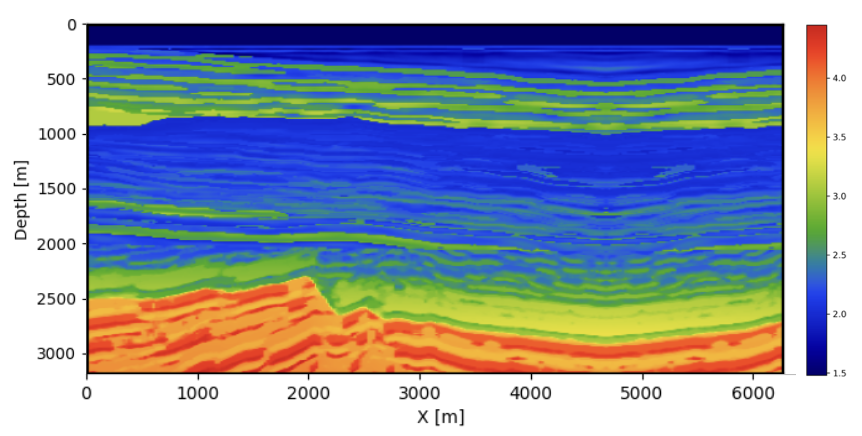

We evaluate the proposed method using 2D slices from the Compass dataset (Jones et al. 2012) to mimic a realistic seismic scenario with distribution shift between acoustic simulations and elastic observations. For the training set, we extract 800 velocity-model slices of size \(6.4\) km \(\times\) \(3.2\) km on a \(512 \times 256\) grid and generate acoustic shot records, which are then migrated using subsurface extensions to form acoustic CIGs used to train the posterior estimator. For a subset of 90 randomly selected models, we instead simulate elastic shot records using the elastic wave equation and then apply the same acoustic migration operator to obtain corresponding CIGs. These elastic-derived CIGs therefore share the same imaging pipeline but originate from elastic wave physics. They are not paired with the acoustic simulations during training and are used only as an unpaired proxy for realistic observations in the MMD-based distribution alignment.
The acquisition geometry consists of 512 equally spaced sources towed at a depth of 12.5 m and 64 ocean-bottom nodes (OBNs) located at jittered horizontal positions (Hennenfent and Herrmann 2008; Herrmann 2010). This jittered sampling scheme follows compressive sensing principles that improve acquisition efficiency (Wason and Herrmann 2013; Oghenekohwo et al. 2017; Wason, Oghenekohwo, and Herrmann 2017; Yin et al. 2023). Seismic wave propagation is simulated with a 15 Hz Ricker wavelet (with energy below 3 Hz tapered for realism) using Devito (Louboutin et al. 2019) and JUDI.jl (Witte et al. 2019). Uncorrelated band-limited Gaussian noise (SNR 12 dB) is added to emulate acquisition noise. To maintain consistency between pressure and particle-velocity observations, the acoustic source is integrated in time as described above. A smooth velocity model, obtained by applying a Gaussian filter with a 5-sample bandwidth to the ground-truth model, is used as a reasonably accurate background model. Finally, 51 horizontal subsurface offsets ranging from \(-500\) m to \(+500\) m are used to construct the CIGs.
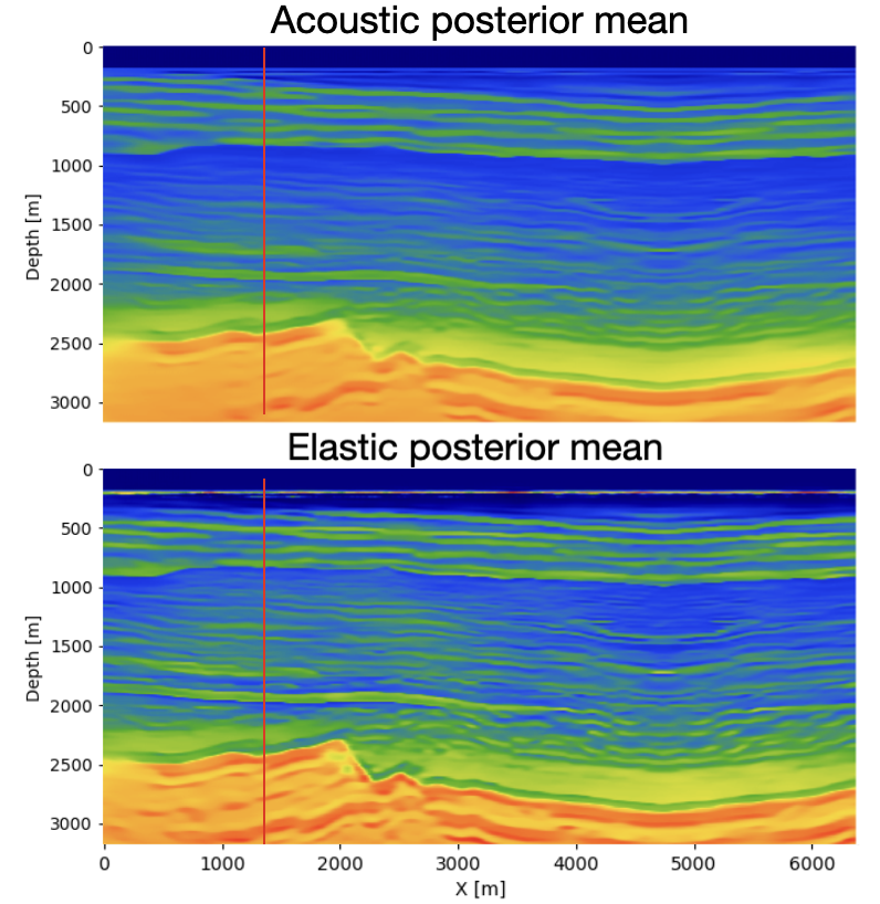
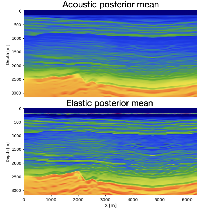
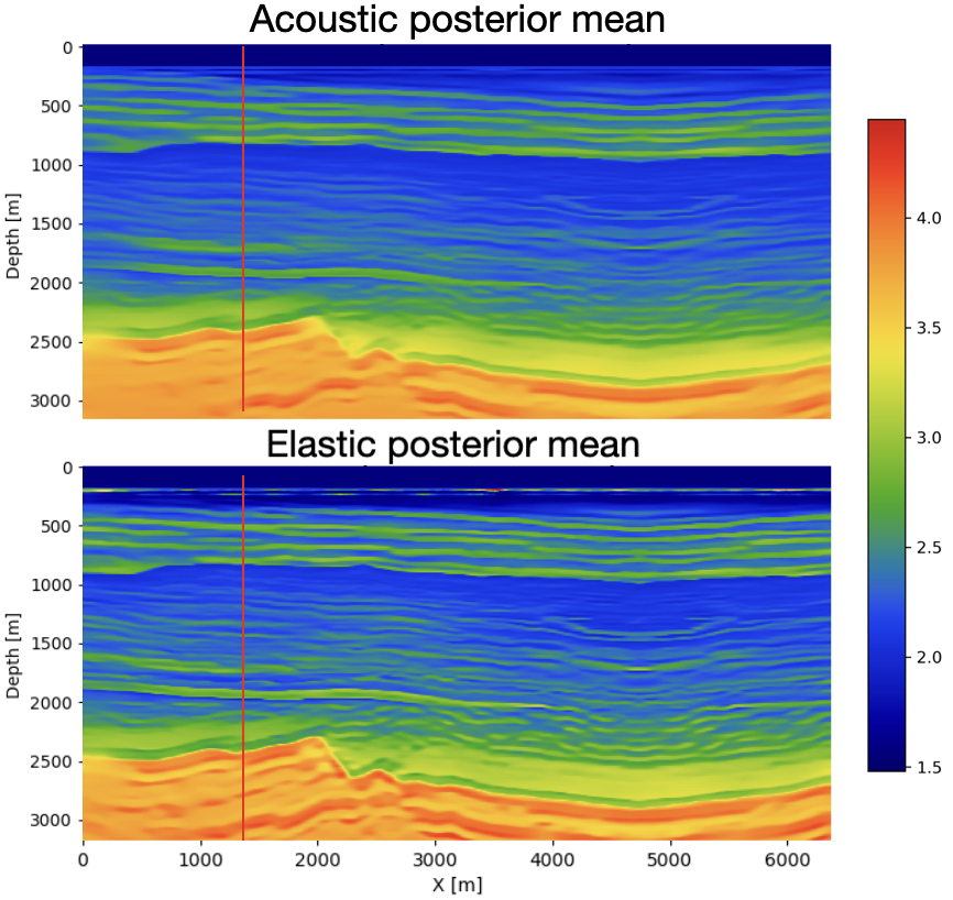
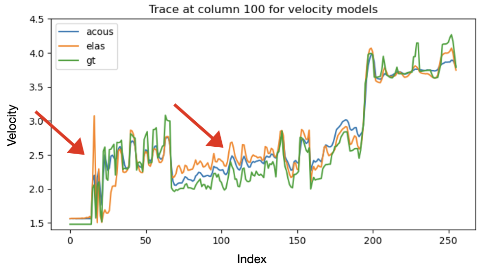
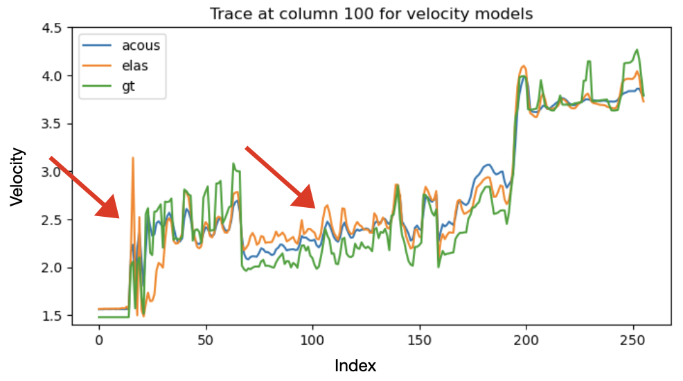
To evaluate the effect of distribution alignment, we test three values of the MMD weight \(\lambda\): (i) \(\lambda=0\), corresponding to no alignment with the elastic distribution; (ii) \(\lambda=1\); and (iii) \(\lambda=10\). figure 1 and figure 2 compare the ground-truth velocity model with the acoustic and elastic posterior means obtained from 64 posterior samples for each \(\lambda\). Across all settings, both acoustic and elastic posteriors recover the large-scale structure of the velocity model, indicating that the summary network extracts the key features relevant for posterior estimation.
For \(\lambda=0\), the elastic posterior mean exhibits several discrepancies relative to the acoustic posterior and the ground truth. First, an abrupt velocity jump appears at approximately 200 m depth, corresponding to the transition from water to unconsolidated sediments.This event is absent in both the ground truth and the acoustic posterior, which likely reflects the large contrast in S-wave velocity across the water bottom. Second, between roughly 1000 m and 2300 m depth, the elastic posterior mean shows consistently higher velocities than both the acoustic posterior and the ground truth. This discrepancy likely reflects additional elastic events generated by S-wave propagation that are not present in acoustic simulations. Third, below 2500 m depth, the elastic posterior resolves slightly finer-scale features than its acoustic counterpart. This may result from PP-reflection amplitudes in the elastic case being influenced by both P- and S-wave velocities, providing richer amplitude information even without MMD regularization.
Introducing the MMD penalty progressively reduces these discrepancies. Both the sharp 200 m contrast and the anomalous mid-depth region become more consistent with the acoustic posterior and the ground truth. This improvement strengthens as \(\lambda\) increases from 1 to 10, demonstrating that stronger MMD regularization brings the elastic summary distribution closer to the acoustic one. To quantify this trend, we compute the structural similarity index measure (SSIM) between each posterior mean and the ground truth and observe a systematic improvement as \(\lambda\) increases.
Seismic traces extracted at \(X=1.4\) km further illustrate this behavior (figure 3). The arrows highlight the water-bottom discontinuity at 200~m depth and the central region of the model. Without MMD (\(\lambda=0\)), the elastic trace deviates substantially from the acoustic and ground-truth traces. With MMD, the elastic trace moves steadily closer to the ground truth by aligning with the acoustic distribution. As \(\lambda\) increases, \(\lambda = 10\), as shown in figure 3, the elastic trace progressively aligns with the acoustic distribution and approaches the ground truth, indicating that the summary network suppresses elastic-specific events that do not inform the P-wave velocity posterior. Notably, the acoustic trace also becomes slightly closer to the ground truth, suggesting a mild mutual-alignment effect induced by MMD.
Overall, these results show that the summary network extracts the most inference-relevant features, and that MMD effectively bridges the distributional gap between simulated acoustic and real elastic data, thereby improving the quality of posterior inference.
CONCLUSION
We introduced ElasNet, a probabilistic framework that bridges acoustic simulations and elastic observations for simulation-based seismic inversion under model misspecification. By combining physics-informed CIG summaries with an attention-based representation and MMD-based distribution alignment, the proposed method enables posterior models trained primarily on inexpensive acoustic simulations to remain consistent with elastic observations.
Synthetic experiments on the Compass dataset show that MMD alignment significantly reduces discrepancies between acoustic and elastic posterior estimates and improves structural similarity. These results demonstrate that robust summary representations combined with distribution alignment provide a practical pathway toward scalable, uncertainty-aware seismic inversion under realistic physics mismatch.
ACKNOWLEDGMENTS
This research was carried out with the support of Georgia Research Alliance and partners of the ML4Seismic Center. During the preparation of this work, the authors used ChatGPT to refine sentence structures and improve the readability of the manuscript. After using this service, the authors reviewed and edited the content as needed and take full responsibility for the content of the publication.