An uncertainty-aware Digital Shadow for underground multimodal CO2 storage monitoring
As a society, we are faced with important challenges to combat climate change. Geological Carbon Storage (GCS), during which gigatonnes of super-critical CO2 are stored underground, is arguably the only scalable net-negative CO2-emission technology that is available. While promising, subsurface complexities and heterogeneity of reservoir properties demand a systematic approach to quantify uncertainty when optimizing production and mitigating storage risks, which include assurances of Containment and Conformance of injected supercritical CO2. As a first step towards the design and implementation of a Digital Twin for monitoring and control of underground storage operations, a machine-learning-based data-assimilation framework is introduced and validated on carefully designed realistic numerical simulations. Because our implementation is based on Bayesian inference, but does not yet support control and decision-making, we coin our approach an uncertainty-aware Digital Shadow. To characterize the posterior distribution for the state of CO2 plumes (its CO2 concentration and pressure), conditioned on multi-modal time-lapse data, the envisioned Shadow combines techniques from Simulation-Based Inference (SBI) and Ensemble Bayesian Filtering to establish probabilistic baselines and assimilate multi-modal data for GCS problems that are challenged by large degrees of freedom, nonlinear multiphysics, non-Gaussianity, and computationally expensive to evaluate fluid-flow and seismic simulations. To enable SBI for dynamic systems, a recursive scheme is proposed where the Digital Shadow’s neural networks are trained on simulated ensembles for their state and observed data (well and/or seismic). Once training is completed, the system’s state is inferred when time-lapse field data becomes available. Contrary to ensemble Kalman filtering, corrections to the predicted simulated states are not based on linear updates, but instead follow during the Analysis step of Bayesian filtering from a prior-to-posterior mapping through the latent space of a nonlinear transform. Starting from a probabilistic model for the permeability field, derived from a baseline surface-seismic survey, the proposed Digital Shadow is validated on unseen simulated ground-truth time-lapse data. In this computational study, we observe that a lack of knowledge on the permeability field can be factored into the Digital Shadow’s uncertainty quantification. Our results also indicate that the highest reconstruction quality is achieved when the state of the CO2 plume is conditioned on both time-lapse seismic data and wellbore measurements. Despite the incomplete knowledge of the permeability field, the proposed Digital Shadow was able to accurately track the unseen physical state of the subsurface throughout the duration of a realistic CO2 injection project. To the best of our knowledge, this work represents the first proof-of-concept of an uncertainty-aware, in-principle scalable, Digital Shadow that captures the uncertainty arising from unknown reservoir properties and noisy observations. This framework provides a foundation for the development of a Digital Twin aimed at mitigating risks and optimizing the management of underground storage projects.
\[ \def\textsc#1{\dosc#1\csod} \def\dosc#1#2\csod{{\rm #1{\small #2}}} \]
1 Introduction
1.1 The need for Geological Carbon Storage
Geological carbon storage (GCS) constitutes capturing carbon dioxide (CO2) emissions from industrial processes followed by storage in deep geological formations, such as depleted oil and gas reservoirs, deep saline aquifers, or coal seams (Page et al. 2020). Because of its ability to scale (Ringrose 2020, 2023), this net-negative CO2-emission technology is widely considered as one of the most promising technologies to help mitigate the effects of anthropogenic CO2 greenhouse gas emissions, which are major contributors to global warming (Bui et al. 2018; IPCC special report 2005). According to the Intergovernmental Panel on Climate Change (IPCC, Panel on Climate Change) (2018)), it is imperative to contain atmospheric warming to \(<2\degree\)C by the year 2100 to avoid serious consequences of global warming. To achieve this goal, scalable net-negative emission technologies that can remove tens of gigatonnes of CO2 per year (IPCC special report 2018) are needed in addition to reducing emissions. These needs call for a transition towards increased use of renewable energy in combination with the global deployment of GCS technology to store significant amounts of supercritical CO2 into geological formations to mitigate the effects of climate change (Metz et al. 2005; Orr Jr 2009). When supercritical CO2—captured at anthropogenic sources (fossil-fuel power plants, steel, cement, and chemical industries), is stored securely and permanently in underground geological storage reservoirs, it can be scaled to mitigate upto \(20\%\) of the total CO2 emission problem (Ketzer, Iglesias, and Einloft 2012). This work is a first step towards an uncertainty-aware Digital Twin aimed at optimizing underground operations while mitigating risks.
1.2 The challenge of monitoring subsurfcae CO2 injection projects
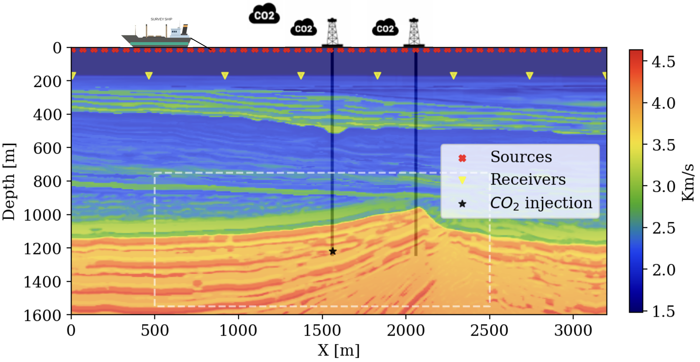
Our main technical objective is directed towards monitoring CO2-storage projects, so that assurances can be made whether storage proceeds as expected and whether CO2 plumes remain within the storage complex. These assurances are referred to as Conformance and Containment by the regulators and operators of GCS (Ringrose 2020, 2023). Even though the proposed methodology could be applied to other settings, our focus is on CO2 storage in offshore saline aquifers in a marine setup as illustrated in figure 1. Compared to storage projects on land, this choice for marine settings circumvents potential complications and risks associated with future liability and geomechanically-induced pressure changes that may trigger earthquakes (Zoback and Gorelick 2012; He et al. 2011; Raza et al. 2016). While this approach simplifies the complexity of underground CO2 storage projects to some degree, simulations for the state of CO2 plumes are on balance more challenging than conventional reservoir simulations because the fluid-flow properties are less well-known. Besides, the process of displacing brine with supercritical CO2 is intricate, taxing multi-phase flow simulators (Ringrose 2020, 2023). To illustrate the possible impact of lack of knowledge on the reservoir properties (the permeability), figure 1 also includes a juxtaposition between multi-phase flow simulations for two different realizations of permeability fields drawn from a stochastic baseline established from active-source surface seismic data (Yin, Orozco, et al. 2024). While both realizations for the permeability are consistent with this baseline, they yield vastly different outcomes where in one case the CO2 plume remains well within (figure 1 bottom-left) the storage complex (denoted by the white dashed line in figure 1) whereas the other simulation obviously breaches Containment (figure 1 bottom-right), due to the presence of an “unknown” high-permeability streak. By maximally leveraging information derived from multimodal time-lapse monitoring data, we plan to guide uncertain reservoir simulations, so outlying “unpredicted” geological events, such as the one caused by the high-permeability streak, can be accounted for.
1.3 Proposed approach with Digital Shadows
As stated eloquently by Ringrose (2020); Ringrose (2023), CO2-storage projects can not rely on static reservoir models alone (Ringrose and Bentley 2016). Instead, reservoir models and simulations need to be updated continuously from multimodal sources (e.g. active-source surface seismic and/or pressure/saturation measurements at wells) of time-lapse data. By bringing this insight together with the latest developments in generative Artificial AI, which includes the sub-discipline of Simulation-Based Inference (SBI, Cranmer, Brehmer, and Louppe (2020)), where conditional neural networks are trained to act as posterior density estimators, and nonlinear ensemble filtering (Spantini, Baptista, and Marzouk 2022), a Digital Shadow (Asch 2022) is coined as a framework for monitoring underground CO2-storage projects. Digital Shadows differ from Digital Twins (Asch 2022) in the sense that they integrate information on the state of a physical object or system — e.g. the temporal behavior of CO2-injection induced changes in pressure/saturation for GCS — by capturing information unidirectionally from real-time, possibly multimodal, observed time-lapse data without feedback loops. While our framework is designed to allow for future optimization, control, and decision-making to mitigate risks of GCS that would turn our Shadow into a Twin, our main focus in this work is to introduce a scalable machine-learning assisted data-assimilation framework (Asch 2022; Spantini, Baptista, and Marzouk 2022). To be relevant to realistic CO2-storage projects, use is made of scalable state-of-the-art reservoir simulation, wave-equation based seismic inversion (Virieux and Operto 2009; Baysal, Kosloff, and Sherwood 1983), ensemble Bayesian filtering (Asch 2022), and the advanced machine-learning technique of neural posterior density estimation (Cranmer, Brehmer, and Louppe 2020; Radev et al. 2020), to capture uncertainties due to our lack of knowledge on the reservoir properties, the permeability field, in a principled way. Because the envisioned Digital Shadow is aimed at monitoring CO2-injection projects over many decades, its performance is validated in silico—i.e. via a well-designed computer-simulation study. As with the development of climate models, this approach is taken by necessity because suitable time-lapse datasets spanning over long periods of time are not yet available.
1.4 Relation to exisiting work
The central approach taken in this work finds its basis in ensemble Kalman Filtering (EnKF, Evensen (1994); Asch, Bocquet, and Nodet (2016); Carrassi et al. (2018)), a widely employed and scalable Bayesian data-assimilation (DA) technique. Here, DA refers to a statistical approach where indirect and/or sparse real-world time-lapse measurements are integrated into a model that describes the dynamics of the hidden state of CO2 plumes. While other time-lapse data-collection modalities exist, including controlled-source electromagnetics (Ayani, Grana, and Liu 2020; Grana, Liu, and Ayani 2021), gravity (Appriou and Bonneville 2022), history matching from data collected at wells (G. Zhang, Lu, and Zhu 2014; Strandli, Mehnert, and Benson 2014), and even tomography with muons (Gluyas et al. 2019), we employ active-source time-lapse surface-seismic surveys (D. E. Lumley 2001) in combination with data collected at wells. Seismic surveys are known for their relatively high attainable resolution, sensitivity to small CO2-induced changes in seismic rock properties, and spatial coverage in both the vertical and horizontal coordinate directions (Ringrose 2020, 2023).
By including crucial multi-phase fluid-flow simulations (Nordbotten and Celia 2011) for the state, and by exchanging the extended Kalman filter (Asch, Bocquet, and Nodet 2016; Asch 2022) for better scalable EnKF (Bruer et al. 2024) type of approach, our work extends early seismic monitoring work by C. Huang and Zhu (2020), where full-waveform inversion (FWI, Virieux and Operto (2009)) is combined with DA. Our choice for a scalable ensemble filtering type of approach (Herrmann 2023; Gahlot et al. 2023; Spantini, Baptista, and Marzouk 2022) is supported by recent work of Bruer et al. (2024), who conducted a careful study on the computational complexity of realistic CO2 projects. This work is aimed at further improving several aspects of ensemble-filter approaches including (i) incorporation of stochasticity in the state dynamics by treating the permeability distribution as a random variable newly drawn after each time-lapse timestep; (ii) removal of reliance on limiting Gaussian assumptions and linearizations of the observation operator; (iii) replacement of the crucial linear Kalman correction step by a learned nonlinear mapping similar to the coupling approach recently proposed by Spantini, Baptista, and Marzouk (2022); and (iv) extending the approach to multimodal time-lapse data.
To meet these additional complexities and evident nonlinearities, we develop a new neural sequential Bayesian inference framework based on Variational Inference (Jordan et al. 1998) with Conditional Normalizing Flows (CNFs, Rezende and Mohamed (2015); Papamakarios et al. (2021); Radev et al. (2020)). As in the work by Spantini, Baptista, and Marzouk (2022), nonlinearities in both the state and observation operators are accounted for by a prior-to-posterior mapping through the latent space of a nonlinear transform, given by a CNF in this work. However, by allowing the permeability field, which emerges in the state for the fluid flow, to appear as a stochastic nuisance parameter, our proposed formulation sets itself apart from existing work. By using the fact that CNFs implicitly marginalize over nuisance parameters during training (Cranmer, Brehmer, and Louppe 2020; Radev et al. 2020), stochasticity due to the lack of knowledge on the permeability field is factored into the uncertainty captured by our neural approximation for the posterior distribution of the CO2 plume’s state.
Finally, the presented approach provides an alternative to “pure” machine-learning approaches, where neural networks are either trained on pairs saturation/seismic shot records (Um et al. 2023), on reservoir models and saturation plumes (Tang et al. 2021), or on “time-lapse movies” (X. Huang, Wang, and Alkhalifah 2024), to produce estimates for the dynamic state with uncertainties based on Mont-Carlo dropout. Aside from the argument that this type of uncertainty quantification may not be Bayesian (Folgoc et al. 2021), our proposed approach is solidly anchored by the fields of DA, where high-fidelity simulations for the state and observations are used to recursively create forecast ensembles, and by SBI (Cranmer, Brehmer, and Louppe 2020; Radev et al. 2020), where advantage is taken of the important concept of summary statistics (Orozco et al. 2023; Orozco, Siahkoohi, et al. 2024) to simplify the complex relationship between the state (saturation/pressure) and seismic observations (shot records). Instead of relying on the network to provide the uncertainty, our deployment of CNFs aims to learn the Bayesian posterior distribution directly that includes both aleatoric, by adding additive noise to the observed time-lapse data, and epistemic uncertainty, by treating the permeability field as a stochastic nuisance parameter. While our approach can be extended to include network-related epistemic uncertainty (Qu, Araya-Polo, and Demanet 2024), we leave this to future work to keep our approach relatively simple.
1.5 Outline
The Digital Shadow for underground CO2-storage monitoring is aimed to demonstrate how learned nonlinear Bayesian ensemble filtering techniques can be used to characterize the state from multimodal time-lapse monitoring data. Our work is organized as follows. In Section 2, we start by introducing the main ingredients of nonlinear ensemble filtering, followed in Section 3 by an exposition on how techniques from amortized Bayesian inference (Cranmer, Brehmer, and Louppe 2020; Radev et al. 2020) can be used to derive our nonlinear extension of ensemble filtering based on CNFs. After specifying algorithms for Sequential Simulation-based Bayesian Inference and \(\textsc{Forecast}\), \(\textsc{Training}\), and \(\textsc{Analysis}\), which includes an introduction of the important aspect of summary statistics, we proceed by illustrating the “lifecycle” of the proposed Digital Shadow, which includes the important prior-to-posterior mapping that corrects the predictions for the state from time-lapse observations. Next, we outline a detailed procedure to validate the proposed Digital Shadow prototype in a realistic off-shore setting representative of the South-Western North Sea. In addition to detailing this setting, which includes descriptions of the probabilistic baseline, ground-truth simulations, and monitoring with the Digital Shadow, Section 4 also introduces certain performance metrics. Guided by these metrics, a case study is presented in Section 5 with an emphasis on examining the advantages of working with multimodal data. This case study is followed by Section 6 in which the Digital Shadow is put in a broader context, followed by conclusions in Section 7.
2 Problem formulation
Monitoring CO2 plumes from multimodal time-lapse measurements from well and/or surface-seismic data calls for an approach where nonlinear causes of epistemic uncertainty, reflecting lack of knowledge on the reservoir properties determining the dynamics, and aleatoric uncertainty, due to noise in the data, are accounted for in a sequential Bayesian inference framework (Tatsis, Dertimanis, and Chatzi 2022; Rubio, Marzouk, and Parno 2023). As a lead into the definition of our Digital Shadow based on amortized neural posterior estimation (Papamakarios and Murray 2016; Lueckmann et al. 2017; Cranmer, Brehmer, and Louppe 2020), we begin by defining general models for nonlinear state dynamics and observations, followed by formulating a general approach to nonlinear Bayesian filtering (Asch 2022).
2.1 Uncertain state dynamics and observation models
While the presented framework is designed to be general, the focus will be on geophysical monitoring of Geological Carbon Storage (GCS) aimed at keeping track of the dynamics of CO2 plumes via a combination of multi-phase flow simulations and time-lapse multimodal geophysical measurements, consisting of sparse localized direct measurements of the saturation and pressure perturbations (shown in figure 12) collected within boreholes of (monitoring) wells and indirect active-source seismic measurements, collected at the surface. In this scenario, the time-varying state-dynamics are measured at discrete time instants, \(k=1\cdots K\), and consists of the time-varying spatial distribution for the CO2 saturation, \(\mathbf{x}_k[S_{\mathrm{CO_2}}]\), and induced pressure perturbation, \(\mathbf{x}_k[\delta p]\), which can be expressed as follows:
\[ \begin{aligned} \mathbf{x}_{k} & = \mathcal{M}_k\bigl(\mathbf{x}_{k-1}, \boldsymbol{\kappa}_k; t_{k-1}, t_k\bigr)\\ & = \mathcal{M}_k\bigl(\mathbf{x}_{k-1}, \boldsymbol{\kappa}_k\bigr),\ \boldsymbol{\kappa}_k\sim p(\boldsymbol{\kappa}) \quad \text{for}\quad k=1\cdots K. \end{aligned} \tag{1}\]
In this expression for the uncertain nonlinear dynamics, the possibly time-dependent dynamics operator, \(\mathcal{M}_k\), represents multi-phase fluid-flow simulations that transition the state from the previous timestep, \(t_{k-1}\), to the next timestep, \(t_k\), for all \(K\) time-lapse timesteps. The dynamics operator, \(\mathcal{M}_k\), which implements the underlying continuous dynamics between times \(t_{k-1}\) and \(t_k\), may itself be time-dependent because of induced chemical and/or rock mechanical changes. Because the spatial distribution of the permeability field, collected in the vector \(\boldsymbol{\kappa}\), is highly heterogeneous (Ringrose 2020, 2023), unknown, and possibly time-dependent, it is treated as a stochastic nuisance parameter (Radev et al. 2020). Without loss of generality, we assume samples for the spatial gridded permeability field to be drawn from the time-invariant probability distribution—i.e, \(\boldsymbol{\kappa}\sim p(\boldsymbol{\kappa})\) where \(p(\boldsymbol{\kappa})\) is assumed to be independent of the state and time-lapse observations. The dynamics operator takes samples from the spatial distribution for the subsurface permeability, \(\boldsymbol{\kappa}\), and the CO2 saturation and reservoir pressure perturbations, collected at the previous timestep \(k-1\) in the vector, \(\mathbf{x}_{k-1}\), as input and produces samples for the CO2 saturation and reservoir pressure perturbations at the next timestep, \(\mathbf{x}_{k}\), as output. While this procedure offers access to samples from the transition density, the transition density itself can not be evaluated because of the presence of the stochastic nuisance parameter, \(\boldsymbol{\kappa}\). To leading order, the nonlinear dynamics consists of solutions of Darcy’s equation and mass conservation laws (Pruess and Nordbotten 2011; Li et al. 2020). Despite the fact that the dynamics can be modeled accurately with reservoir simulations (Krogstad et al. 2015; Settgast et al. 2018; Rasmussen et al. 2021; Stacey and Williams 2017), relying on these simulations alone is unfeasible because of a lack of knowledge on the permeability.
To improve estimates for the state, CO2 plumes are monitored by collecting discrete time-lapse well (Freifeld et al. 2009) and surface-seismic data (D. Lumley 2010). We model these multimodal time-lapse datasets as
\[ \mathbf{y}_k = \mathcal{H}_k(\mathbf{x}_k,\boldsymbol{\epsilon}_k, \mathbf{\bar{m}}_k),\ \boldsymbol{\epsilon}_k \sim p(\boldsymbol{\epsilon}) \quad\text{for}\quad k=1,2,\cdots,K \tag{2}\]
where the vector, \(\mathbf{y}_k\), represents the observed multimodal data at timestep \(k\). To add realism, the seismic data is corrupted by the noise term, \(\boldsymbol{\epsilon}_k\), sampled by filtering realizations of standard zero-centered Gaussian noise with a bandwidth-limited seismic source-time function. This filtered noise is normalized to attain a preset signal-to-noise ratio before it is added to the seismic shot records prior to reverse-time migration. The shot records themselves are generated with 2D acoustic simulations with the seismic properties (velocity and density) linked to the CO2 saturation through the patchy saturation model1 (Avseth, Mukerji, and Mavko 2010). The vector, \(\mathbf{\bar{m}_k}=(\mathbf{\bar{v}}, \mathbf{\bar{\rho}})\) with \(\mathbf{\bar{v}}\) and \(\mathbf{\bar{\rho}}\) the reference velocity and density, represents a time-dependent seismic reference model from which the migration-velocity model for imaging will be derived and with respect to which the time-lapse differences in the seismic shot records will be calculated. According to these definitions, the observation operator, \(\mathcal{H}_k\), models multimodal, direct and indirect, time-lapse monitoring data, collected at the (monitoring) wells and migrated from surface-seismic shot records. While this observation operator may also depend on time, e.g. because the acquisition geometry changes, we assume it, like the dynamics operator, to be time-invariant, and drop the time index \(k\) from the notation.
Due to sparsely sampled receiver and well locations, and the non-trivial null-space of the modeling operators, the above measurement operator is ill-posed, which renders monitoring the CO2 dynamics challenging, a situation that is worsened by the intrinsic stochasticity of the dynamics. To overcome these challenges, we introduce a nonlinear Bayesian filtering framework where the posterior distribution for the state, conditioned on the collected multimodal time-lapse data, is approximated by Variational Inference (Jordan et al. 1999; David M. Blei and McAuliffe 2017) with machine learning (Rezende and Mohamed 2015; Siahkoohi et al. 2023b; Orozco, Siahkoohi, et al. 2024), neural posterior density estimation to be precise. With this approach, which combines the latest techniques from sequential Bayesian inference and amortized neural posterior density estimation (Papamakarios et al. 2021), we aim to quantify the uncertainty of the CO2 plumes in a principled manner.
2.2 Nonlinear Bayesian filtering
Because both the dynamics and observation operators are nonlinear, we begin by defining a general probabilistic model for the state and observations in terms of the following conditional distributions:
\[ \mathbf{x}_k \sim p(\mathbf{x}_k\mid\mathbf{x}_{k-1}) \tag{3}\]
and
\[ \mathbf{y}_k \sim p(\mathbf{y}_k\mid\mathbf{x}_{k}), \tag{4}\]
for \(k=0\cdots K\), representing, respectively, the transition density, defined by equation 1, and the data likelihood, given by equation 2. These conditional distributions hold because the above monitoring problem (cf. equations 1 and 2) is Markovian, which implies that the likelihood does not depend on the time-lapse history—i.e., \(\left(\mathbf{y}_k\perp\mathbf{y}_{1:k-1}\right)\mid\mathbf{x}_k\) with the shorthand, \(\mathbf{y}_{1:k}= \left\{\mathbf{y}_1,\ldots,\mathbf{y}_k\right\}\), so that \(p(\mathbf{y}_k\mid \mathbf{x}_k, \mathbf{y}_{1:k-1})=p(\mathbf{y}_k\mid \mathbf{x}_k)\). This orthogonality assumption holds as long as the nuisance parameters are independent with respect to the state (Rubio, Marzouk, and Parno 2023). The aim of Bayesian filtering is to recursively compute the posterior distribution of the state at time, \(k\), conditioned on the complete history of collected time-lapse data—i.e., compute \(p(\mathbf{x}_k\mid \mathbf{y}_{1:k})\). There exists a rich literature on statistical inference for dynamical systems (McGoff, Mukherjee, and Pillai 2015) aimed to accomplish this goal, which entails the following three steps (Asch 2022):
Initialization step: Choose the prior distribution for the state \(p(\mathbf{x}_0)\).
Prediction step: Compute the predictive distribution for the state derived from the Chapman-Kolmogorov equation yielding (Tatsis, Dertimanis, and Chatzi 2022)
\[ \begin{aligned} p(\mathbf{x}_k\mid \mathbf{y}_{1:k-1})&=\int p(\mathbf{x}_k\mid \mathbf{x}_{k-1})p(\mathbf{x}_{k-1}\mid \mathbf{y}_{1:k-1})\mathrm{d}\mathbf{x}_{k-1}\\ & = \mathbb{E}_{\mathbf{x}_{k-1}\sim p(\mathbf{x}_{k-1}\mid\mathbf{y}_{1:k-1})}\bigl[p(\mathbf{x}_{k}\mid\mathbf{x}_{k-1})\bigr]. \end{aligned} \tag{5}\]
This step uses equation 1 to advance samples of the distribution \(p(\mathbf{x}_{k-1}\mid \mathbf{y}_{1:k-1})\) to samples of \(p(\mathbf{x}_k\mid \mathbf{y}_{1:k-1})\).
Analysis step: Apply Bayes’ rule
\[ p(\mathbf{x}_{k}|\mathbf{y}_{1:k}) \propto p(\mathbf{y}_{k}|\mathbf{x}_{k}) p(\mathbf{x}_{k}|\mathbf{y}_{1:k-1}) \tag{6}\]
with \(p(\mathbf{y}_{k}|\mathbf{x}_{k})\) and \(p(\mathbf{x}_k\mid \mathbf{y}_{1:k-1})\) acting as the “likelihood” and “prior”. During this step, the posterior distribution is calculated by correcting the “prior” with the “likelihood”. To this end, equation 4 will be used to draw samples from the likelihood.
These three steps are general and make no assumptions on the linearity and Gaussianity of the distributions involved. The general solution of the above Bayesian filtering problem is far from trivial for the following reasons: (i) equations 5 and 6 only permit analytical solutions in cases where the state-dynamics and observation operators are linear and Gaussian distributed; (ii) the presence of the nuisance permeability parameter in equation 1 requires access to the marginal likelihood, which is computationally infeasible (Cranmer, Brehmer, and Louppe 2020; Kruse et al. 2021a); (iii) likewise, the marginalization in equation 5 is also not viable computationally; and finally (iv) computing the above conditional probabilities becomes intractable in situations where the state is high dimensional and the state-dynamics and observational operators are computationally expensive to evaluate.
To address these challenges, numerous data-assimilation techniques have been developed over the years (Asch, Bocquet, and Nodet 2016). The ensemble Kalman filter (EnKF) (Evensen 1994; Carrassi et al. 2018) features amongst the most advanced techniques and is widely used for large nonlinear state-space and observation models. During the prediction step of the data-assimilation recursions, EnKF propagates a set of \(M\) particles from the previous timestep, \(\left\{\mathbf{x}^{(1)}_{k-1},\ldots,\mathbf{x}^{(M)}_{k-1}\right\}\), to the next timestep by applying the state-space dynamics (equation 1) to each particle, followed by generating simulated observation samples, \(\left\{\mathbf{y}^{(1)}_{k},\ldots,\mathbf{y}^{(M)}_{k}\right\}\), based on the observation model of equation 2. During the subsequent analysis step, EnKF uses the pairs, \(\{\mathbf{x}_k^{(m)}, \mathbf{y}_k^{(m)}\}_{m=1}^M\), to calculate empirical Monte-Carlo based linear updates to the forecast ensemble. While EnKF avoids the need for linearization, calculation of gradients, and is relatively straightforward to scale, it relies on linear updates that prevent it from solving the above nonlinear and non-Gaussian Bayesian filtering problem accurately, even when increasing the ensemble size (Spantini, Baptista, and Marzouk 2022).
Instead of relying on linear mappings, we consider the analysis step in equation 6 as a trainable prior-to-posterior transformation and employ techniques from amortized neural posterior density estimation with CNFs (Kruse et al. 2021b; Gahlot et al. 2023; Herrmann 2023) to carry out the analysis step, an approach also taken by Spantini, Baptista, and Marzouk (2022), who proposes a closely related but different coupling technique. Our proposed approach derives from simulation-based inference (Cranmer, Brehmer, and Louppe 2020; Radev et al. 2020) with invertible CNFs, which extends EnKF by allowing for learned nonlinear prior-to-posterior density transformations. CNFs represent a class of invertible neural networks that, dependent on a condition term, convert samples from a complicated distribution, through a series of nonlinear differentiable transformations, into samples from a simpler distribution, e.g. the standard Gaussian distribution. Instead of explicit evaluations of the corresponding densities, and similar to EnKF workflows, access is only needed to samples from the “likelihood” and “prior”, available through simulations with equations 1 and 2.
3 Methodology
To free ourselves from limiting assumptions, which either rely on simplifying linearity and Gaussianity assumptions or on computationally unfeasible Markov chain Monte-Carlo (McMC) based approaches, extensive use will be made of Variational Inference (VI) (Jordan et al. 1999) with CNFs (Rezende and Mohamed 2015; Ardizzone et al. 2019a; Kruse et al. 2021a). In these approaches, scalable optimization techniques are used to match parametric representations of distributions with CNFs to unknown target distributions. During simulation-based inference (SBI) (Cranmer, Brehmer, and Louppe 2020; Radev et al. 2020), the forward Kullback-Leibler (KL) divergence (Kullback and Leibler 1951; Siahkoohi et al. 2023a) is minimized on samples from the joint distribution for the state and observations, which involves a relatively easy to evaluate quadratic objective function. In this approach, the CNFs correspond to generative neural networks that serve as conditional density estimators (Radev et al. 2020) for the posterior distribution. After explaining the training and inference phases of SBI, the technique of sequential simulation-based inference will be introduced. This technique is designed to serve as a nonlinear extension of EnKF. To this end, algorithms for the recurrent \(\textsc{Forecast}\), \(\textsc{Training}\), and \(\textsc{Analysis}\) stages of the proposed neural Bayesian filtering approach will be presented.
3.1 Amortized Bayesian Inference with CNFs
Recent developments in generative Artificial Intelligence (genAI), where neural networks are trained as surrogates for high-dimensional (conditional) distributions, are key to the development and success of our uncertainty-aware Digital Shadow, which relies on capturing the posterior distribution from simulated samples for the state and observations. While any amortized neural network implementation capable of producing samples conditioned on samples for different observations will work in our setting, and this includes conditional neural networks based on conditional score-based diffusion (Batzolis et al. 2021), CNFs have our preference because they allow us to quickly sample from the posterior, \(\mathbf{x}\sim p(\mathbf{x}\mid\mathbf{y})\), and conduct density calculations—i.e., evaluate the posterior density \(p(\mathbf{x}\mid\mathbf{y})\) and its derivatives with respect to the states, \(\mathbf{x}\), and observations, \(\mathbf{y}\). This latter feature is necessary when designing Digital Twins capable of uncertainty-informed decisions (Alsing, Edwards, and Wandelt 2023), control (Gahlot et al. 2024), and Bayesian experimental design (Orozco, Herrmann, and Chen 2024). While non-amortized approaches may be feasible, amortization of the neural estimate of the posterior distribution is essential because it allows us to marginalize over stochastic nuisance parameters (the permeability field, \(\boldsymbol{\kappa}\), in our case) while capturing its uncertainty from the ensemble of dynamic states and associated time-lapse observations.
Specifically, our goal is to capture the posterior distribution from pairs, \(\{\mathbf{x}^{(m)}, \mathbf{y}^{(m)}\}_{m=1}^M\) (time-dependence was dropped for simplicity). To achieve this goal, we make use of Bayesian Variational Inference (Rezende and Mohamed 2015) in combination with the ability to carry out simulations of the state dynamics and observations (cf. equations 1 and 2), which are of the type (Radev et al. 2020)
\[ \mathbf{y}=\mathcal{G}(\mathbf{x},\boldsymbol{\zeta})\quad\text{with}\quad \boldsymbol{\zeta}\sim p(\boldsymbol{\zeta}\mid\mathbf{x}),\, \mathbf{x}\sim p(\mathbf{x}) \tag{7}\]
where \(\mathcal{G}\) is a generic simulator that depends on samples of the prior, \(\mathbf{x}\sim p(\mathbf{x})\), and nuisance parameters, \(\boldsymbol{\zeta}\sim p(\boldsymbol{\zeta}\mid\mathbf{x})\), possibly conditioned on samples of the prior. These simulated samples give us implicit access to the likelihood. Given \(M\) sampled pairs, \(\{\mathbf{x}^{(m)}, \mathbf{y}^{(m)}\}_{m=1}^M\), simulation-based inference with CNFs proceeds by training an invertible neural network to approximate the posterior distribution, \(p(\mathbf{x}\mid\mathbf{y})\), by minimizing the forward Kullback–Leibler (KL) divergence between the true and the approximate posterior for all possible data, \(\mathbf{y}\). The training objective reads (Radev et al. 2020; Siahkoohi et al. 2023a)
\[ \begin{aligned} \widehat{\boldsymbol{\phi}}&= \mathop{\mathrm{argmin}\,}\limits_{\boldsymbol{\phi}}\mathbb{E}_{p(\mathbf{y})}\bigl[\mathbb{KL}\bigl(p(\mathbf{x}\mid \mathbf{y})\mid\mid p_{\boldsymbol{\phi}}(\mathbf{x}\mid \mathbf{y})\bigr)\bigr]\\ & =\mathop{\mathrm{argmin}\,}\limits_{\boldsymbol{\phi}}\mathbb{E}_{p(\mathbf{y})}\Bigl[\mathbb{E}_{p(\mathbf{x}\mid\mathbf{y})}\bigl[-\log p_{\boldsymbol{\phi}}(\mathbf{x}\mid\mathbf{y})+p(\mathbf{x}\mid\mathbf{y})\bigr]\Bigr] \\ & = \mathop{\mathrm{argmax}\,}\limits_{\boldsymbol{\phi}}\mathbb{E}_{p(\mathbf{x},\mathbf{y})}\bigl[\log p_{\boldsymbol{\phi}}(\mathbf{x}\mid\mathbf{y})\bigr]. \end{aligned} \tag{8}\]
To arrive at this objective involving samples from the joint distribution for \(\mathbf{x}\) and \(\mathbf{y}\), use was made of the law of total probability that allows us to rewrite the marginalization over observations, \(\mathbf{y}\), in terms of the expectation over samples from the joint distribution. The term \(p(\mathbf{x}\mid\mathbf{y})\) can be dropped because it does not depend on the parameters, \(\boldsymbol{\phi}\). For more details, see Siahkoohi et al. (2023a). The above objective is used to approximate the true posterior distribution as accurately as possible, \(p_{\boldsymbol{\phi}}(\mathbf{x}\mid\mathbf{y})\approx p(\mathbf{x}\mid\mathbf{y})\) for all possible \(\mathbf{x}\) and \(\mathbf{y}\), drawn from the joint distribution, \(p(\mathbf{x},\mathbf{y})\). Following Radev et al. (2020), the approximate posterior, \(p_{\boldsymbol{\phi}}(\mathbf{x}\mid\mathbf{y})\) is parameterized with a conditional Invertible Neural Network (cINN, Ardizzone et al. (2019a)), \(f_{\boldsymbol{\phi}}\), which conditioned on, \(\mathbf{y}\), defines an invertible mapping.
With the change-of-variable rule of probability
\[ p_{\boldsymbol{\phi}}(\mathbf{x}\mid\mathbf{y})=p\bigl(\mathbf{z}=f_{\boldsymbol{\phi}}(\mathbf{x};\mathbf{y})\bigr)\Bigl |\det\Bigl(\mathbf{J}_{f_{\boldsymbol{\phi}}}\Bigr)\Bigr | \]
with \(\mathbf{J}_{f_{\boldsymbol{\phi}}}\) the Jacobian of \(f_{\boldsymbol{\phi}}\) evaluated at \(\mathbf{x}\) and \(\mathbf{y}\), the objective of maximizing the likelihood in equation 8 becomes
\[ \begin{aligned} \widehat{\boldsymbol{\phi}}&=\mathop{\mathrm{argmax}\,}\limits_{\boldsymbol{\phi}}\mathbb{E}_{p(\mathbf{x},\mathbf{y})}\bigl[\log p_{\boldsymbol{\phi}}(\mathbf{x}\mid\mathbf{y})\bigr]\\ &= \mathop{\mathrm{argmax}\,}\limits_{\boldsymbol{\phi}}\mathbb{E}_{p(\mathbf{x},\mathbf{y})}\Bigl[\log p\bigl(\mathbf{z}=f_{\boldsymbol{\phi}}(\mathbf{x};\mathbf{y})\bigr)+\log\Bigl |\det\Bigl(\mathbf{J}_{f_{\boldsymbol{\phi}}}\Bigr)\Bigr |\Bigr]. \end{aligned} \tag{9}\]
Given the simulated training pairs, \(\{\mathbf{x}^{(m)}, \mathbf{y}^{(m)}\}_{m=1}^M\), maximization of the expectations in equation 9 can be approximated by minimization of the sum:
\[ \begin{aligned} \widehat{\boldsymbol{\phi}}&= \mathop{\mathrm{argmin}\,}\limits_{\boldsymbol{\phi}}\frac{1}{M}\sum_{m=1}^M \Bigl(-\log p\bigl(f_{\boldsymbol{\phi}}(\mathbf{x}^{(m)};\mathbf{y}^{(m)})\bigr)-\log\Bigl |\det\Bigl(\mathbf{J}^{(m)}_{f_{\boldsymbol{\phi}}}\Bigr)\Bigr |\Bigr)\\ & =\mathop{\mathrm{argmin}\,}\limits_{\boldsymbol{\phi}} \frac{1}{M}\sum_{m=1}^M \Biggl(\frac{\Big\|f_{\boldsymbol{\phi}}(\mathbf{x}^{(m)};\mathbf{y}^{(m)})\Big\|_2^2}{2} - \log\Bigl |\det\Bigl(\mathbf{J}^{(m)}_{f_{\boldsymbol{\phi}}}\Bigr)\Bigr |\Biggr). \end{aligned} \tag{10}\]
During derivation of this training loss for CNFs, use was made of the property: \(\mathcal{N}(0,\mathbf{I})\propto \exp(-(1/2)\|\mathbf{z}\|_2^2)\). In the ideal situation where the estimated network weights, \(\widehat{\boldsymbol{\phi}}\), attain a global minimum of the objective in equation 8, the latent distribution will be statistically independent of the conditioning data (Radev et al. 2020). In that case, samples from the posterior can be drawn based on the following equivalence:
\[ \mathbf{x}\sim p_{\widehat{\boldsymbol{\phi}}}(\mathbf{x}\mid\mathbf{y}) \,\Longleftrightarrow\, f^{-1}_{\widehat{\boldsymbol{\phi}}}(\mathbf{z};\mathbf{y})\sim p(\mathbf{x}\mid\mathbf{y})\quad\text{with}\quad \mathbf{z}\sim \mathcal{N}(0,\mathbf{I}). \tag{11}\]
According to this equivalence, sampling from the posterior corresponds to generating samples from the multidimensional standard Gaussian distribution, \(\mathbf{z}\sim \mathcal{N}(0,\mathbf{I})\), followed by computing \(f^{-1}_{\widehat{\boldsymbol{\phi}}}(\mathbf{z};\mathbf{y})\). In the next section, we will employ and adapt these training and inference phases for the less-than-ideal recursive training regime of data-assimilation problems where the ensemble sizes are relatively small for which the global minimum of equation 8 may not be attained.
3.2 Neural sequential simulation-based inference
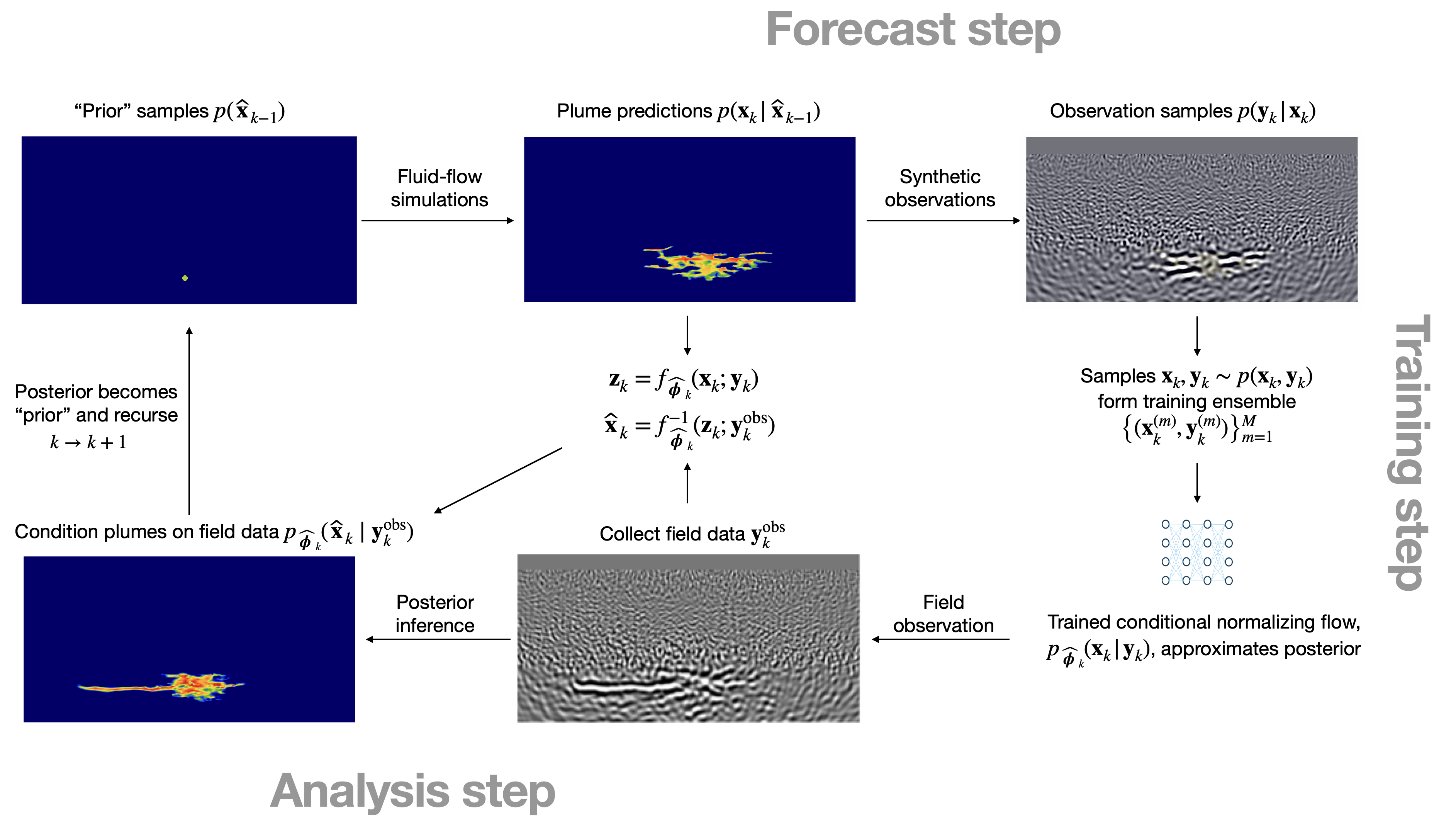
After randomized initialization of \(M\) particles of the CO2 plume’s initial state, \(\widehat{\mathbf{x}}^{(m)}_0\sim p(\mathbf{x}_0)\) (line 2 of Algorithm 1), training pairs for the state (equation 1) and observations (equation 2), \(\{\mathbf{x}_k^{(m)},\mathbf{y}_k^{(m)} \}_{m=1}^{M}\), for the next time step, are predicted by simulations with the state dynamics and detailed in the \(\textsc{Forecast}\) step of Algorithm 2). For notational convenience, we already introduced the symbol, \(\widehat{\quad}\), to distinguish between predicted “digital states” and analyzed predictions (denoted by the \(\widehat{\quad}\)) for the state conditioned on the field observed data. During the \(\textsc{Forecast}\) step of Algorithm 2, random samples of the stochastic permeability field and noise are drawn and used to draw samples from the transition density (line 3 of Algorithm 2), conditioned on analyzed samples, \(\{\widehat{\mathbf{x}}_k^{(m)}\}_{m=1}^M\), from the previous time step. These predictions for the advanced state are subsequently employed to sample observations (line 4 of Algorithm 2), producing the simulated training ensemble, \(\{\mathbf{x}_k^{(m)},\mathbf{y}_k^{(m)} \}_{m=1}^{M}\). These simulated pairs are utilized during the \(\textsc{Training}\) step (line 6 of Algorithm 1) where equation 10 is minimized with respect to the CNF’s network weights, yielding \(\widehat{\boldsymbol{\phi}}_k\). Given these network weights, \(M\) latent-space representations for each pair are calculated via
\[ \mathbf{z}_k^{(m)}= f_{\widehat{\boldsymbol{\phi}}_k}(\mathbf{x}_k^{(m)};\mathbf{y}_k^{(m)}), \tag{12}\]
for \(m=1\cdots M\) (Spantini, Baptista, and Marzouk 2022). Given observed field data, \(\mathbf{y}_k^{\mathrm{obs}}\), collected at time \(k\) (line 7 of Algorithm 1), these latent variables are used to correct the state for \(m=1\cdots M\) via
\[ \widehat{\mathbf{x}}_k^{(m)}= f^{-1}_{\widehat{\boldsymbol{\phi}}_k}(\mathbf{z}_k^{(m)};\mathbf{y}_k^{\mathrm{obs}}). \tag{13}\]
In this expression, \(\{\widehat{\mathbf{x}}_k^{(m)}\}_{m=1}^M\), corresponds for \(k\geq 1\) to analyzed states, produced by the prior-to-posterior mapping (Algorithm 2 in Spantini, Baptista, and Marzouk (2022)). To offset the potential effects of working with a limited ensemble size, \(M\), we choose to adapt this approach of producing samples from the latent space calculated from the forecast ensemble. According to Spantini, Baptista, and Marzouk (2022), this process mitigates the effects when a global minimum of equation 10 is not attained, implying that \(p_{\widehat{\boldsymbol{\phi}}}(\mathbf{z})\perp \mathbf{x}\) may no longer hold. In that case, the latent output distribution is no longer guaranteed to be the same for any fixed, \(\mathbf{y}\) (Radev et al. 2020). By producing latent samples that derive directly from the predicted state-observation pairs, this issue is resolved. When conditioned on the observed field data, \(\mathbf{y}_k^{\mathrm{obs}}\), these latent samples improve the inference after running the CNF in the reverse direction (cf. equation 13). Algorithm 2 summarizes the three key phases, namely the \(\textsc{Forecast}\), \(\textsc{Training}\), and \(\textsc{Analysis}\) steps, which are used during the recursions in Algorithm 1 that approximate equations 5 and 6. During these recursions, for timesteps \(k>1\), samples of the posterior distribution from the previous timestep, \(\{\widehat{\mathbf{x}}^{(m)}_{k-1}\}_{m=1}^M\), serve as “priors” for the next timestep, producing, \(\{\widehat{\mathbf{x}}^{(m)}_k\}_{m=1}^M\), which are conditioned on the observations, \(\mathbf{y}_k^{\mathrm{obs}}\). This procedure corresponds to the nonlinear prior-to-posterior of Spantini, Baptista, and Marzouk (2022).
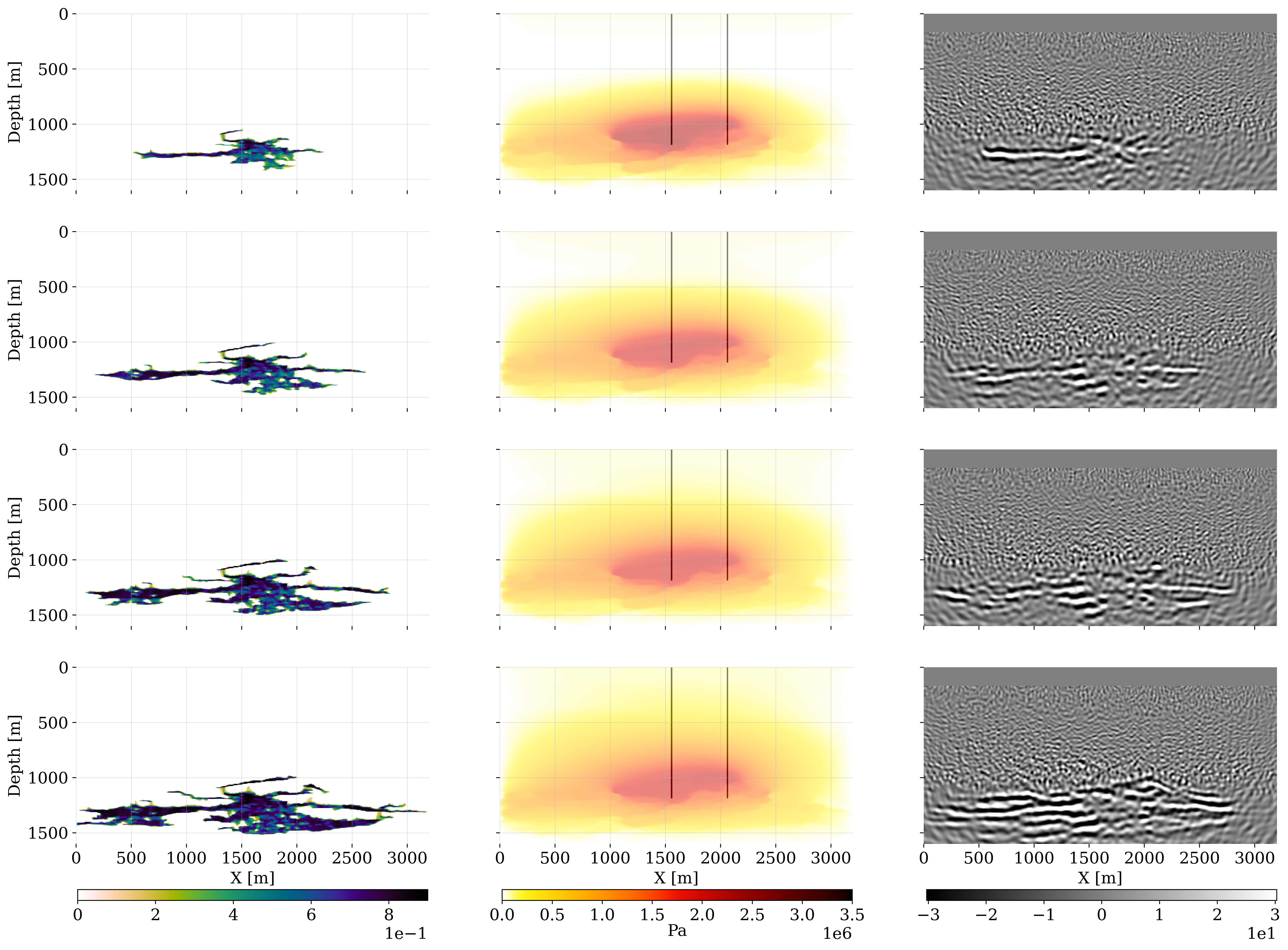
To illustrate the different stages of the Digital Shadow’s recursions, figure 2 is included to depict its “lifecycle” at the first timestep, \(k=1\). The lifecycle entails the following stages. Samples for the initial state of the CO2 saturation, denoted with a slight abuse of notation by \(\widehat{\mathbf{x}}^{(m)}_0\sim p(\mathbf{x}_0)\), are drawn first from the uniform distribution, \(\widehat{\mathbf{x}}^{(m)}_0\sim \mathcal{U}(0.1,\, 0.6)\) (figure 2 (top-left)). By simulating the state-dynamics equation 1 (figure 2 top-row middle), predictions for the state at the next timestep are sampled, \(\mathbf{x}_{k}\sim p(\mathbf{x}_{k}| \widehat{\mathbf{x}}_{k-1})\). Given these predicted samples for the state, corresponding samples for the observations are simulated with equation 2 (figure 2 top-row right). These two types of simulations make up the \(\textsc{Forecast}\) step, which produces the predicted training ensemble, \(\bigl\{\mathbf{x}_{k}, \mathbf{y}_{k}\bigr\}_{m=1}^M\), consisting of \(M\) samples drawn from the joint distribution, \(\mathbf{y}_{k}\sim p(\mathbf{x}_{k}, \mathbf{y}_{k})\). This predicted ensemble serves as input to the \(\textsc{Training}\) step (figure 2 bottom right) during which the weights of the Digital Shadow’s neural networks are trained by minimizing equation 9. This produces the optimized network weights, \(\widehat{\boldsymbol{\phi}}_k\), at timestep, \(k\). After collecting field observations, \(\mathbf{y}_k^{\mathrm{obs}}\), posterior inference is conducted with the neural posterior density estimator, \(p_{\widehat{\boldsymbol{\phi}}_k}(\widehat{\mathbf{x}}_{k} \mid\mathbf{y}_{k}^{\mathrm{obs}})\), conditioned on the observed field data, \(\mathbf{y}_k^{\mathrm{obs}}\). To avoid finite sample size and training effects during the \(\textsc{Analysis}\) step (figure 2 lower left), a sample from the posterior is drawn by evaluating the CNF in the forward latent-space direction on the predicted pair, \((\mathbf{x}_{k}, \mathbf{y}_{k})\), yielding \(\mathbf{z}_k = f_{\widehat{\boldsymbol{\phi}}_k}(\mathbf{x}_k;\mathbf{y}_k)\). This operation is followed by running the CNF, conditioned on the observed field data, \(\mathbf{y}_{k}^{\mathrm{obs}}\), in the reverse direction, yielding the sample \(\widehat{\mathbf{x}}_k= f^{-1}_{\widehat{\boldsymbol{\phi}}_k}(\mathbf{z}_k;\mathbf{y}_k^{\mathrm{obs}})\). By design, this sample approximates a sample from the true posterior, \(\mathbf{x}_k\sim p(\mathbf{x}_k\mid \mathbf{y}_k^{\mathrm{obs}})\). At the next timestep, this sample becomes a sample for the “prior”—i.e., for \(k\rightarrow k+1\), and the recursions proceed by repeating themselves for all, \(K\), timesteps. By comparing figure 2’s sample for the plume prediction, \(\mathbf{x}_{k}\sim p(\mathbf{x}_{k}| \widehat{\mathbf{x}}_{k-1})\), with the corresponding analyzed sample conditioned on the observed field data, \(\widehat{\mathbf{x}}_{k} \sim p_{\widehat{\boldsymbol{\phi}}_k}(\widehat{\mathbf{x}}_{k} \mid\mathbf{y}_{k}^{\mathrm{obs}})\), it becomes apparent that the predicted state produced by the \(\textsc{Forecast}\) step undergoes a significant correction during the \(\textsc{Analysis}\) step. This mapping during the \(\textsc{Analysis}\) step between the predicted and inferred states—i.e., \(\mathbf{x}_k\mapsto \widehat{\mathbf{x}}_k\), derives from the invertibility of CNFs and the implicit conditioning of the predictions on \(\mathbf{y}^{\mathrm{obs}}_{k-1}\) (via \(\widehat{\mathbf{x}}_{k-1}\)) and explicit conditioning on \(\mathbf{y}^{\mathrm{obs}}_k\). Despite the fact that the state at the previous timestep is conditioned on \(\mathbf{y}^{\mathrm{obs}}_{k-1}\), the prediction varies considerably. This variability is caused by the unknown permeability field, which appears as a stochastic nuisance parameter in the dynamics (cf. equation 1), and explains the significant time-lapse data-informed correction performed by the \(\textsc{Analysis}\) step. The importance of the correction is nicely illustrated by the example in figure 2 where thanks to the correction the plume is extended significantly in the leftward direction, a feature completely missed by the predicted state.
By running through the Digital Shadow’s lifecycle \(k\) times recursively for an ensemble consisting of \(M\) particles, the \(\textsc{Prediction}\) and \(\textsc{Analysis}\) steps approximate samplings from \(p(\mathbf{x}_k\mid \mathbf{y}^{\mathrm{obs}}_{1:k-1})\) and \(p(\mathbf{x}_k\mid \mathbf{y}^{\mathrm{obs}}_{1:k})\) of equations 5 and 6. Because the proposed posterior density estimation scheme recurrently trains networks, it can be considered as an instance of neural sequential Bayesian inference, which forms the basis of our Digital Shadow. Before going into further details on how the simulations are performed, we introduce the important concept of summary statistics, which simplifies the observable-to-state mapping, renders typically non-uniform seismic data space uniform, and also learns to detect features that inform the posterior.
3.3 Physics-based summary statistics
Despite the adequate expressiveness of CNF’s neural architecture based on cINNs (Ardizzone et al. 2019b), the mapping of CO2 plume-induced acoustic changes to seismic shot records remains extremely challenging because of the large degrees of freedom of Earth models and seismic shot records (Cranmer, Brehmer, and Louppe 2020), which live in three dimensions and five dimensions for 2- and 3D- Earth models, respectively. This challenge is compounded by the relatively weak signal strength of time-lapse changes, the complexity of the time-lapse changes to seismic observations map, and the fact that raw seismic shot records are collected non-uniformly—i.e. different seismic surveys may have different numbers of shot records or shot records may vary in the number of traces (receivers), time samples, etc. To overcome these issues, we introduce a hybrid approach, consisting of physics-based summary statistics (Radev et al. 2020; Orozco et al. 2023), and a trainable U-net (Ronneberger, Fischer, and Brox 2015) that forms the conditional arm of the cINN (Ardizzone et al. 2019a). By mapping the shot records to the image domain, uniformity is assured because the discretization can be controlled in that domain. Moreover, the mapping from the image domain to the velocity model is much simpler, so the conditional arm of the cINN can dedicate itself to learning image-domain features that maximally inform the posterior while the network’s invertible arm can concentrate on learning how to produce samples of the posterior from realizations of standard Gaussian noise conditioned on these features. More importantly, Alsing, Wandelt, and Feeney (2018) also showed that under certain conditions the gradient of the score function (the \(\log\)-likelihood) compresses physical data optimally. Motivated by this work, Orozco et al. (2023) demonstrated that information in the original shot records can be preserved during pre-stack reverse-time migration (RTM) as long as the migration-velocity model is sufficiently accurate. Yin, Orozco, et al. (2024) showed that this condition can be relaxed in the WISE and WISER (Yin, Orozco, and Herrmann 2024) frameworks. The network weights for the U-net in the conditional arm are absorbed in the network weights, \(\boldsymbol{\phi}\), of the CNFs, and trained during the minimization of the objective in equation 10.
To meet the challenges of imaging subtle time-lapse changes induced by the replacement of brine by supercritical CO2, we calculate the residual with respect to a reference model, \(\mathbf{\bar{m}}_k\). To avoid tomographic artifacts in the gradient, the residual is migrated with the inverse-scattering imaging condition (Stolk, Hoop, and Op’t Root 2009; Douma et al. 2010; Whitmore and Crawley 2012; P. Wang et al. 2024). This corresponds to computing sensitivities with respect to the acoustic impedance for a constant density. Given this choice, the observation operator linking the state of the CO2 plume to migrated time-lapse seismic images is given by
\[ \begin{aligned} \mathbf{y}_k&=\mathcal{H}_k(\mathbf{x}_k,\boldsymbol{\epsilon}_k, \mathbf{\bar{m}}_k)\\ &:=\Bigl({\mathbf{J}_{\mathcal{F}[\mathbf{v}]}}\Bigr |_{{\mathbf{\widetilde{v}}_k}}\Bigr)_{\mathsf{ic}}^{\top} \Bigl(\mathcal{F}[\mathbf{\bar{m}}_k]-\mathbf{d}_k\Bigr) \end{aligned} \tag{14}\]
In this expression, the linear operator \(\Bigl({\mathbf{J}_{\mathcal{F}[\mathbf{v}]}}\Bigr |_{{\mathbf{\widetilde{v}}_k}}\Bigr)_{\mathsf{ic}}\) corresponds the Jacobian of the forward wave operator, \(\mathcal{F}[\mathbf{m}]\), calculated at \(\mathbf{\widetilde{v}}_k\), which is a smoothed version of the reference velocity model, \(\mathbf{\bar{v}_k}\). The symbol \(^\top\) denotes the adjoint. Together with the reference densities, the reference wavespeeds are collected in the seismic reference model, \(\bar{\mathbf{m}}_k\). The nonlinear forward model, \(\mathcal{F}\), represents the active-source experiments part of the survey. Use of the inverse-scattering imaging condition is denoted by the subscript, \(\mathsf{ic}\) in the definition of the reverse-time migration operator, \(\Bigl({\mathbf{J}_{\mathcal{F}[\mathbf{v}]}}\Bigr |_{{\mathbf{\widetilde{v}}_k}}\Bigr)^\top_{\mathsf{ic}}\). Finally, the vector, \(\mathbf{d}_k\), collects the simulated shot records at time-lapse timestep, \(k\), for all active-source experiments and is simulated with
\[ \mathbf{d}_k=\mathcal{F}[\mathbf{m}_k]+\boldsymbol{\epsilon}_k,\quad \text{where} \quad \mathbf{m}_k = \mathcal{R}({\mathbf{m}_0, \mathbf{x}_k}). \tag{15}\]
In this nonlinear forward model at timestep, \(k\), the CO2saturation induced corrected time-lapse seismic medium properties—i.e., the wavespeed, \(\mathbf{v}_k\), and the density, \(\boldsymbol{\rho}_k\), are computed with respect to the baseline, \(\mathbf{m}_0\), via \(\mathbf{m}_k = \mathcal{R}({\mathbf{m}_0, \mathbf{x}_k})\). This nonlinear operator, \(\mathcal{R}(\cdot,\cdot)\), captures the rock physics, which models how changes in the state—i.e., the CO2 saturation, map to changes in the seismic medium properties, \(\mathbf{m}_k\). Because “observed field” seismic time-lapse data is assumed to come from the same forward model, equation 14 will also be used to in silico simulate \(\mathbf{y}_k^{\mathrm{obs}}\), simply by replacing the simulated time-lapse shot records, \(\mathbf{d}_k\), by the simulated observed time-lapse seismic shot records, \(\mathbf{d}_k^{\mathrm{obs}}\), that stand for data collected in the field.
Given the exposition of the amortized Bayesian inference, the neural sequential simulation-based Bayesian inference, and physics-based summary statistics, we are now in a position to setup our Digital Shadow for GCS prior to conducting our case study.
4 Digital Shadow for CO2 storage monitoring
To validate our Digital Shadow, an in silico prototype is developed and implemented for the off-shore setting of the South-Western North Sea, an area actively considered for GCS (ETI 2016). For this purpose, we consider the 2D cross-section of the Compass model (E. Jones et al. 2012) and the experimental setup of figure 1, which consists of sparse ocean-bottom nodes, dense sources, an injection, and a monitor well. Based on the velocity model in figure 1, a probabilistic model for reservoir properties (permeability) will be derived first, followed by the establishment of the ground truth for the in sillico simulated states and associated observed time-lapse seismic and well data, which serve as input to our Digital Shadow for CO2 storage monitoring.
4.1 Probabilistic baseline model for the permeability field
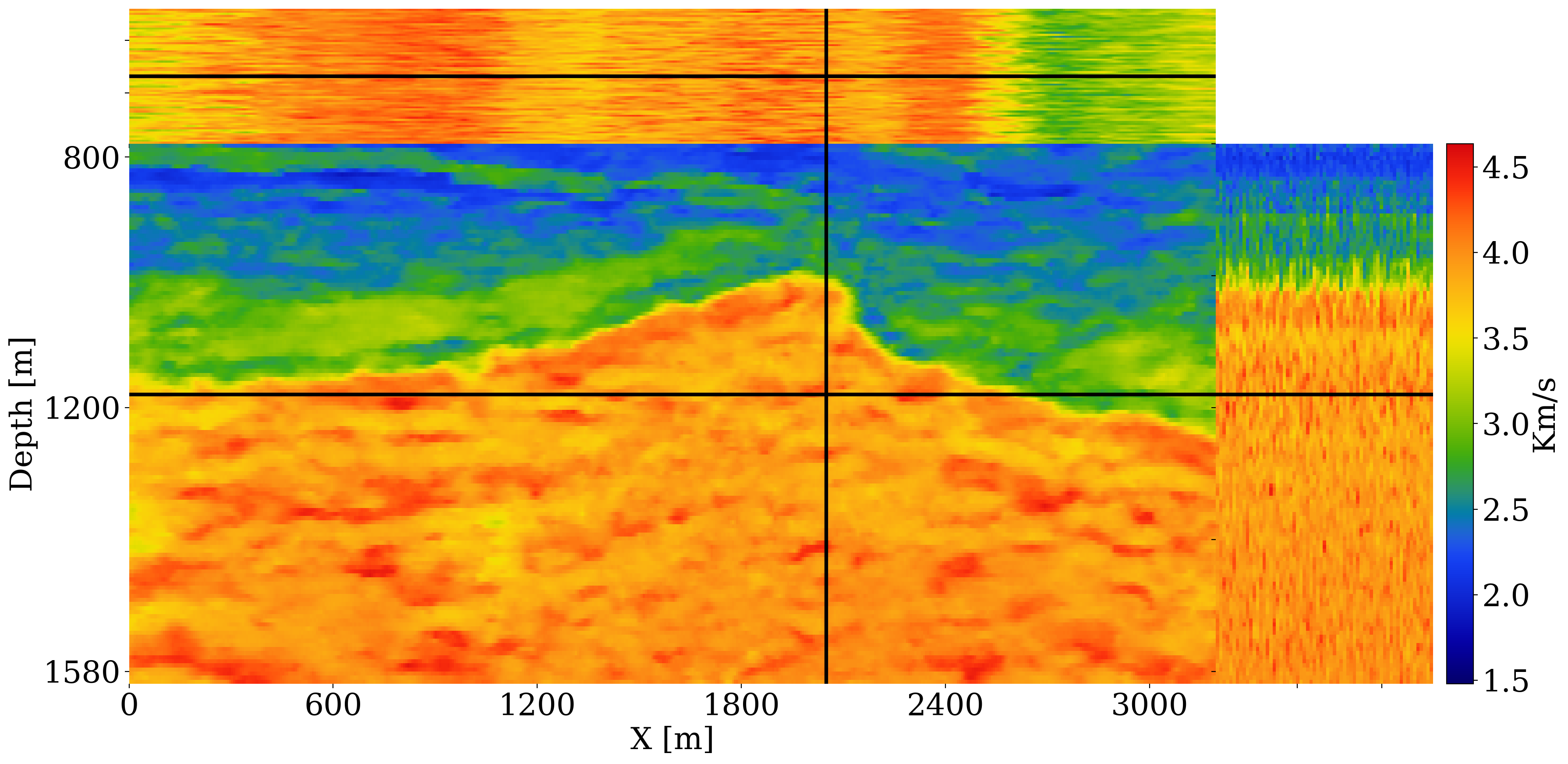
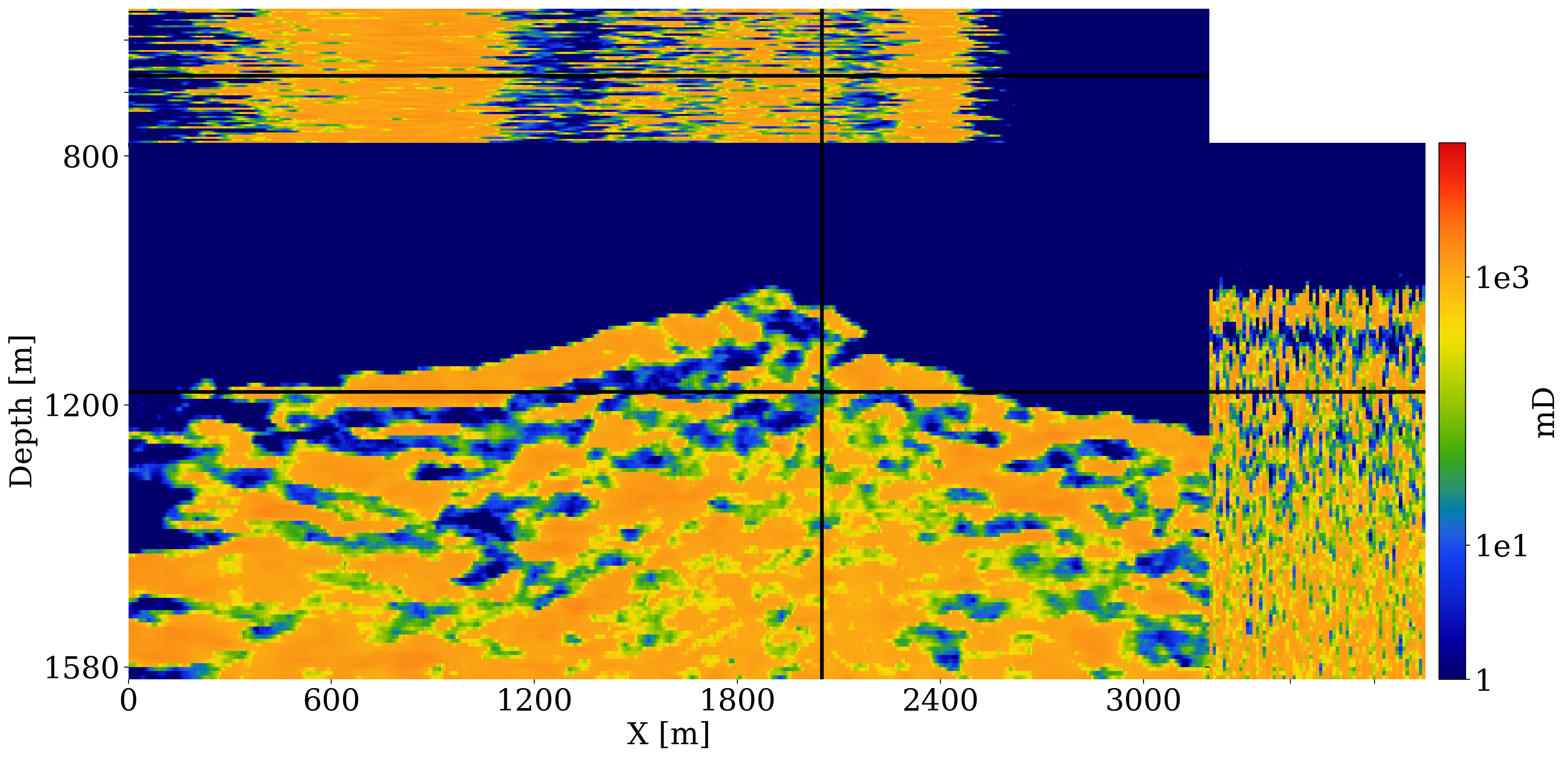
To mimic a realistic CO2 storage project where reservoir properties are not known precisely, a stochastic baseline for the permeability field is established. To this end, the velocity model depicted in figure 1 is used to generate noisy baseline seismic data (signal-to-noise ratio S/N \(12\mathrm{dB}\)). This seismic baseline dataset serves as input to full-waveform variational Inference via Subsurface Extensions (WISE (Yin, Orozco, et al. 2024)). Given a poor 1D migration-velocity model and noisy shot records, WISE draws samples from the posterior distribution for the velocity. These samples for the wavespeed conditioned on shot data are plotted in figure 3 (a) and are converted to the permeability fields plotted in figure 3 (b). This elementwise velocity-to-permeability conversion is done with the following nonlinear elementwise mapping:
\[ \boldsymbol{\kappa}=\begin{cases} \boldsymbol{\zeta}\odot\exp_\circ(\mathbf{v}-4.5)\oslash \exp_\circ(4.0-4.3) \quad &\mathrm{if}\quad \mathbf{v}\succcurlyeq 4.0\\ 0.01 \exp_\circ\bigl((\log_\circ (\boldsymbol{\zeta}/0.01)/0.5)\odot(\mathbf{v}-3.5)\bigr) \quad &\mathrm{if}\quad \mathbf{v}\succcurlyeq 3.5 \\ 0.01\exp_\circ(\mathbf{v}-1.5)\oslash\exp_\circ(3.5-1.5) \quad &\mathrm{else.} \end{cases} \tag{16}\]
In this expression, the symbols \(\odot\),\(\oslash\), \(\exp_\circ\), and \(\log_\circ\), refer to elementwise multiplication, division, exponentiation, and logarithm. The conversion itself consists of elementwise exponential scaling and randomization with \(\boldsymbol{\zeta}\sim\mathrm{smooth}\bigl(\mathcal{N}(1000, 1200)\bigr)\), where is \(\boldsymbol{\zeta}\) a realization of the standard Normal distribution smoothed with Gaussian kernel of width \(5\mathrm{m}\). The conversion is also controlled by elementwise (denoted by the elementwise greater or equal symbol \(\succcurlyeq\)) operations, which involve the wavespeeds. These inequalities are chosen such that the permeability values are high (between \(1600 \mathrm{mD}\) and \(3000 \mathrm{mD}\)) for regions where the wavespeeds are above \(4.0\mathrm{km/s}\). These regions correspond to clean sandstones. Areas with wavespeeds that vary within the interval \(3.5-4.0\mathrm{km/s}\) stand for dirty sands with intermediate permeability values between \(10 \mathrm{mD}\) and \(1600 \mathrm{mD}\) while areas with lower wavespeeds correspond to shales with the lowest permeability values of \(0.001 \mathrm{mD}\).
Because of the noise and poor migration-velocity model, the samples for the baseline velocity models produced by WISE (see figure 3 (a) for a subset of these samples) exhibit strong variability. This variability amongst the samples of the baseline \(\mathbf{v}\sim p(\mathbf{v}\mid \mathbf{y}_0^{\mathrm{obs}})\) produces, after conversion by equation 16, highly variable samples for the permeability field, \(\boldsymbol{\kappa}\sim p(\boldsymbol{\kappa})\), included in figure 3 (b). Because the permeability values are small to extremely small in the primary and secondary seals, they are denoted by solid blue-color overburden areas in figure 3 (b). These plots exhibit high variability, especially in areas where the permeable sandstones are interspersed with low-permeable shales and mudstones. This high degree of variability in the permeability field reflects our lack of knowledge of this crucial reservoir property, which complicates CO2 plume predictions based on reservoir simulations alone. Our Digital Shadow is aimed at demonstrating how time-lapse data can be used to condition the simulations, so the ground-truth CO2 plume can be estimated more accurately from monitoring data.
Geologically, the considered CO2-injection site corresponds to a proxy for a storage complex in the South-Western corner of the North Sea with a reservoir made of a thick stack of relatively clean highly-permeable Bunter sandstone (Kolster et al. 2018). The study area corresponds to a 2D slice selected from the synthetic Compass model (E. Jones et al. 2012), which itself was created from imaged seismic and well-log data collected in a region under active consideration for Geological Carbon Storage (GCS) by the North-Sea Transition Authority (ETI 2016). The seals of the storage complex comprise the Rot Halite Member, as a primary seal about \(50 \mathrm{m}\) thick, situated directly on top of the Blunt sandstone, and the Haisborough Group, as the secondary seal over \(300\mathrm{m}\) thick consisting of low-permeability mudstones.
The velocities of the 3D Compass model were also used to train the networks of WISE (Yin, Orozco, et al. 2024). The reader is referred to Yin, Orozco, et al. (2024) for further details on the training of these neural networks. To create a ground-truth dataset, our simulation-based workflow follows the numerical case study by Erdinc et al. (2022) and Yin, Erdinc, et al. (2023), where realistic time-lapse seismic surveys were generated in response to CO2 injection in a saline aquifer.
4.2 In silico ground-truth simulations
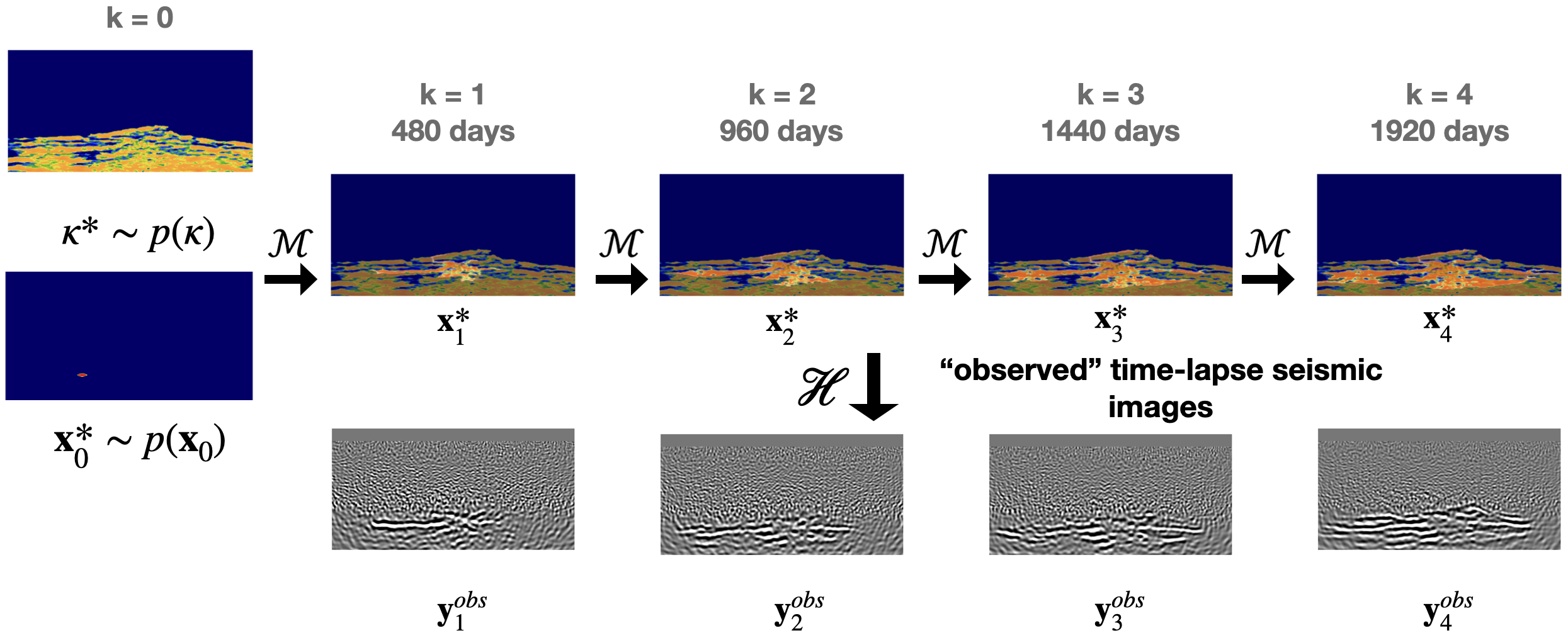
The Digital Shadow will be validated against unseen ground-truth multimodal simulations. At this early stage of development, we opt for in silico simulations for the ground-truth CO2-plume dynamics and the seismic images of the induced time-lapse changes. This choice, which is not an uncommon practice in areas such as climate modeling where future data does not exist, also offers more control and the ability to validate with respect to a ground truth to which there is no access in practice. The fluid-flow simulations themselves are carried out over \(24\) timesteps of \(80\) days each. The time-lapse seismic images are derived from four sparsely sampled noisy ocean-bottom node surveys, collected over a period of \(1920=4\times 480\) days.
4.2.1 Multi-phase flow simulations
Figure 4 contains a schematic overview on how the ground-truth flow simulations are initialized by randomly sampling the ground-truth (denoted by the symbol \(^\ast\)) permeability field, \(\boldsymbol{\kappa}^\ast\), and the initial state for the CO2 plume at timestep, \(k=0\)—i.e. the CO2 saturation is sampled, \(\widehat{\mathbf{x}}^{\ast}_0\sim \mathcal{U}(0.2,\, 0.6)\). The ground-truth anisotropic permeability field, \(\boldsymbol{\kappa}\), consists of \(512\times 256\) gridpoints with a grid spacing of \(6.25\mathrm{m}\) and has a vertical-to-horizontal permeability ratio of \(\kappa_v/\kappa_h = 0.36\). The reservoir extends \(100\mathrm{m}\) in the perpendicular \(y\)-direction. Supercritical CO2 is injected at a depth of \(1200\mathrm{m}\) over an injection interval of \(37.5 \mathrm{m}\) for the \(1920\) day duration of the project with an injection rate of \(0.0500\mathrm{m^3/s}\), pressurizing the reservoir from a maximum pressure of \(9.7e6\) to \(1.1e7\mathrm{Pa}\). The total amount of injected CO2 is \(5.8 \mathrm{Mt}\) with \(1.1. \mathrm{Mt}\) injected annually. The hydrostatic pressure at the injection depth of \(1200\mathrm{m}\) is well below the depth at which CO2 becomes critical.
The resulting multi-phase fluid-flow simulations (Nordbotten and Celia 2011) by the reservoir simulator (Krogstad et al. 2015; Settgast et al. 2018; Rasmussen et al. 2021; Stacey and Williams 2017; Møyner et al. 2024) are collected in the vector, \(\mathbf{x}^\ast_{1:24}\), see figure 4 top-row for the time-lapse states, \(\mathbf{x}^\ast_{1:6:24}\) (\(1:6:24\) means taking each \(6^{\mathrm{th}}\) sample). The simulations themselves are conducted with an implicit method implemented with the open-source software package JutulDarcy.jl (Møyner and Bruer 2023). This industry-scale reservoir modeling package simulates how the injected CO2 gradually displaces brine within the connected pore space of rocks in the storage complex. Initially, the reservoir rocks are filled with brine. Both brine and CO2 residual saturations are set to \(10\%\) each. As can be seen from figure 4, the CO2 plume follows regions of high permeability, forming extensive fingers in the lateral direction. Because the density of critical CO2 is smaller than that of brine (\(700\mathrm{kg/m^3}\) for CO2 versus \(1000\mathrm{kg/m^3}\) for water) buoyancy effects drive the CO2 plume upwards.
4.2.2 Seismic simulations
To convert changes in the reservoir’s state due to CO2 injection to modifications in the seismic properties, a nonlinear rock physics model, \(\mathcal{R}\), is introduced as in Yin, Erdinc, et al. (2023) and Louboutin, Yin, et al. (2023). At each of the \(K=4\) time-lapse time instances, changes in the CO2 saturation are related to differences in the seismic properties by this model. When ignoring velocity changes due to pressure changes and assuming a heterogeneous distribution of the CO2, the patchy saturation model (Avseth, Mukerji, and Mavko 2010) can be used to relate increases in CO2 saturation to reductions in the acoustic wavespeed and density. Given baseline wavespeeds and densities gathered in the seismic medium properties vector, \(\mathbf{m}_0=(\mathbf{v}_0,\boldsymbol{\rho}_0)\), the rock physics at each timestep, \(k\), reads
\[ \mathbf{m}_k=\mathcal{R}(\mathbf{m}_0,\mathbf{x}_k),\, k=1\cdots K. \tag{17}\]
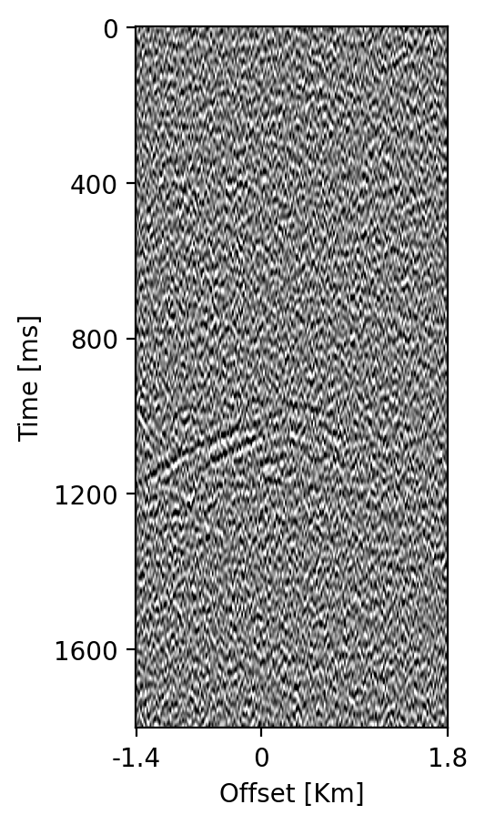
Figure 5 includes an example of how changes in the CO2 saturation at timestep, \(k=1\), are mapped to changes in the acoustic wavespeed and density. In turn, these time-lapse changes in the seismic properties lead to changes in the simulated shot records as shown in figure 6, which depicts time-lapse seismic differences with respect to data generated with the reference model for \(k=1\cdots 4\). Shot records are simulated by solving the acoustic wave equation for varying density and acoustic wavespeeds using the open-source software package JUDI.jl, a Julia Devito Inversion framework (P. A. Witte et al. 2019; Louboutin, Witte, et al. 2023), which uses highly optimized time-domain finite-difference propagators of Devito (Louboutin et al. 2019; Luporini et al. 2020).
The four ground-truth time-lapse seismic surveys are generated after \(480, 960, 1440, \mathrm{and}\, 1920\) days since the start of the CO2 injection. There is no free surface. Throughout the fixed acquisition setup, \(200\) shot records with airgun locations sampled at \(16\mathrm{m}\) interval are collected sparsely by eight Ocean Bottom Nodes (OBNs) with a receiver interval of \(400\mathrm{m}\), yielding a maximum offset of \(3.2\mathrm{km}\). During the seismic simulations, a Ricker wavelet with a dominant frequency of \(15\mathrm{Hz}\) is used, and band-limited noise with a signal-to-noise ratio (SNR) of \(28.0 \mathrm{dB}\) is added to the \(1800\mathrm{ms}\) recordings sampled at \(4\mathrm{ms}\). Due to the complexity of the model and time-lapse changes, the time-lapse differences with respect to the reference model are noisy and have normalized root-mean-square (NRMS) values of \(2.65,\, 4.60,\, 4.60\) and \(4.61\) after \(480, 960, 1440, \mathrm{and}\, 1920\) days.
Ground-truth time-lapse shot records, \(\mathbf{d}^{\mathrm{obs}}_{1:K}\) serve as input to the time-lapse imaging scheme, detailed below, which produces the ground-truth time-lapse images, \(\mathbf{y}^{\mathrm{obs}}_{1:K}\), depicted in the bottom row of figure 4. Despite the strong artifacts, consisting of epistemic linearization errors and aleatoric observation noise, these time-lapse seismic images display a distinct imprint of the growing CO2 plume. How these images are formed and used to condition estimates for the dynamic state, will be discussed next.
4.3 CO2 monitoring with the Digital Shadow
Amortized posterior inference stands at the basis of our Digital Shadow. As described in Section 3.1, training CNFs requires the creation of predicted training ensembles during the \(\textsc{Forecast}\) step, which consists of input-output pairs made out of samples from the “prior” and “likelihood”. Forming these ensembles is followed by the \(\textsc{Training}\) step during which the network weights are calculated. Neural inference happens at the final \(\textsc{Analysis}\) step during which members of the predicted ensemble for the state are corrected by measurements from the field, \(\mathbf{y}^{\mathrm{obs}}_{k}\). After exhaustive testing, the size of the ensemble was chosen to be \(M=128\), a number that will be used throughout our experiments. Aside from determining the ensemble size, this number also determines how Monte-Carlo estimates the conditional mean
\[ \mathbf{\bar{x}}= \mathbb{E}_{ p(\mathbf{x}\mid\mathbf{y})} \left[ \mathbf{x}\right]\approx \frac{1}{M}\sum_{m=1}^M\mathbf{x}^{(m)}\quad \tag{18}\]
and conditional variance
\[ \boldsymbol{\bar{\sigma}}^2 = \mathbb{E}_{ p(\mathbf{x}\mid\mathbf{y})} \Bigl[\bigl(\mathbf{x} - \mathbb{E}_{ p(\mathbf{x}\mid\mathbf{y})} \bigr )^2\Bigr] \approx \frac{1}{M}\sum_{m=1}^M\bigl(\mathbf{x}^{(m)}-\mathbf{\bar{x}}\bigr)^2 \tag{19}\]
are calculated.
4.3.1 The Forecast step
The creation of realistic simulation-based ensembles forms a crucial part of our Digital Shadow. Details on how these training ensembles for the Digital Shadow are assembled are provided next.
Uncertain dynamics
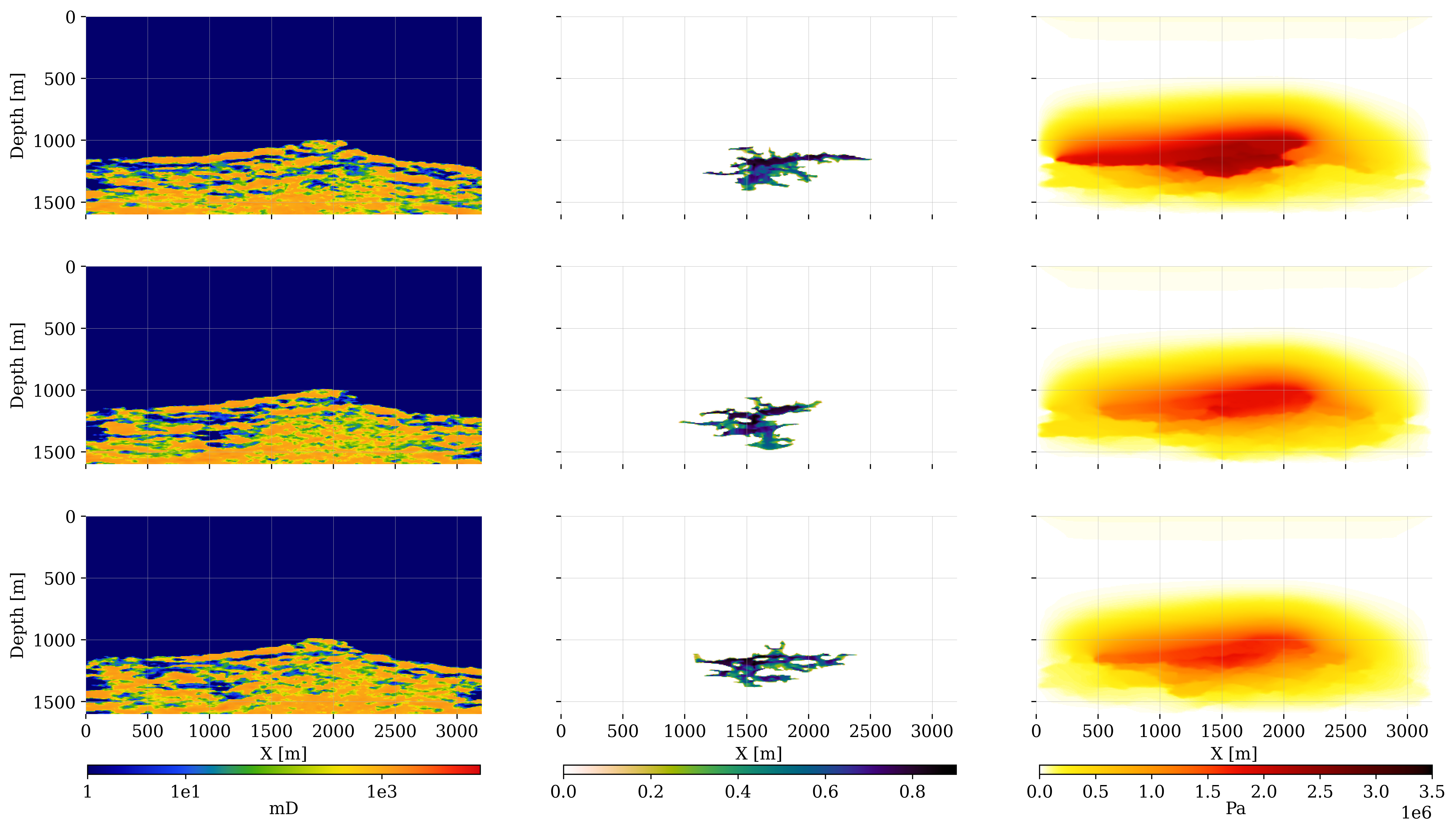
The main purpose of the Digital Shadow for CO2 monitoring lies in its ability to handle uncertainties, in particular epistemic uncertainty due to the unknown permeability field, which throughout the simulations for the dynamics is considered as a random vector (cf. equation 1). This implies that during each evaluation of the dynamics, \(\mathcal{M}\), a new sample for the permeability field is drawn, \(\boldsymbol{\kappa}_k\sim p(\boldsymbol{\kappa})\), according the procedure describe in Section 4.1. Because the high-permeability zones differ between samples, the injection depth varies between \(1200-1250\mathrm{m}\). As can be seen from figure 7, the variability amongst the permeabilities, injection depth, and initial saturation, are all responsible for the variable CO2 plume predictions, even after a single timestep at time \(k=1\). Both the CO2 saturation and pressure perturbations differ for each permeability realization. The predicted CO2 saturations have complex shapes that vary significantly. The pressure perturbations vary less, are smooth, and as expected cover a larger area.
Seismic reference model
While the different realizations for the permeability field give rise to different CO2 saturations, revealing their time-lapse seismic signature calls for a dedicated RTM imaging procedure with migration-velocity models, \(\widetilde{\mathbf{v}}_k\), that are corrected at each time-lapse timestep, and with residuals that are computed with respect to a carefully chosen reference model. To derive these migration-velocity and reference models, the forecast ensemble for the state, \(\{\mathbf{x}^{(m)}_k\}_{m=1}^M\), is used to update the seismic properties with equation 17. Given this predicted ensemble for the state, the seismic properties and simulated shot records are given by
\[ \mathbf{m}_k^{(m)} = \mathcal{R}({\mathbf{{m}}_0}, \mathbf{x}_k^{(m)})\quad \text{and}\quad \mathbf{d}_k^{(m)} = \mathcal{F}(\mathbf{m}_k^{(m)})+\boldsymbol{\epsilon}_k,\quad m=1\cdots M, \tag{20}\]
by virtue of equation 15.
Since the time-lapse changes are small, and epistemic and aleatoric uncertainties significant, the challenge is to define for each time-lapse survey an appropriate reference velocity model. This reference model serves two purposes. First, it is used to generate reference shot records with respect to which the time-lapse differences are calculated. Second, after smoothing, it yields migration-velocity models, \(\widetilde{\mathbf{v}}_k\), for each timestep.
To compute this reference model, the seismic properties for the baseline, \(\mathbf{m}_0\), are updated with the rock physics model, \(\mathbf{\bar{m}}_k = \mathcal{R}({\mathbf{{m}}_0}, \mathbf{\bar{x}}_k)\) where \(\mathbf{\bar{x}}_k=\frac{1}{M}\sum_{m=1}^M\mathbf{x}_k^{(m)}\) is the average state at timestep \(k\). From these reference models, \(\mathbf{\bar{m}}_k\), the corresponding migration-velocity models, \(\widetilde{\mathbf{v}}_k\), are obtained via smoothing. Using equation 14, the migrated images for the ensemble are now computed as follows:
\[ \begin{aligned} \mathbf{y}_k^{(m)}&=\mathcal{H}(\mathbf{x}_k^{(m)},\boldsymbol{\epsilon}_k, \mathbf{\bar{m}}_k)\\ &:=\bigl({\mathbf{J}_{\mathcal{F}[\mathbf{v}]}}\Bigr |_{{\mathbf{\widetilde{v}}_k}}\bigr)_{\mathsf{ic}}^{\top} \Bigl(\mathcal{F}[\mathbf{\bar{m}}_k]-\mathbf{d}_k^{(m)}\Bigr), \quad m=1\cdots M. \end{aligned} \tag{21}\]
In this expression, seismic images for each ensemble member are calculated by migrating differences between shot records computed in the reference model and shot records of the ensemble given by equation 20 with a migration-velocity model that is given by \(\widetilde{\mathbf{v}}_k\). Because the surveys are replicated, the time-lapse time-index subscript in the observation operator is dropped.
With the uncertain dynamics and observation operators in place, we are after initialization (lines 1—3 of Algorithm 1) ready to execute the \(\textsc{Forecast}\) step (cf. Algorithm 2 line 5). During this \(\textsc{Forecast}\) step, tuples \(\{\mathbf{x}_k^{(m)},\mathbf{y}_k^{(m)} \}_{m=1}^{M}\) are produced that serve as input to the CNF training. By replacing the simulated ensemble shot records with the ground-truth “field” shot records, \(\mathbf{d}^{\mathrm{obs}}_k\), in equation 21, the observed images, \(\mathbf{y}^{\mathrm{obs}}_k\), introduced in Section 4.2 are formed.
4.3.2 The Training step
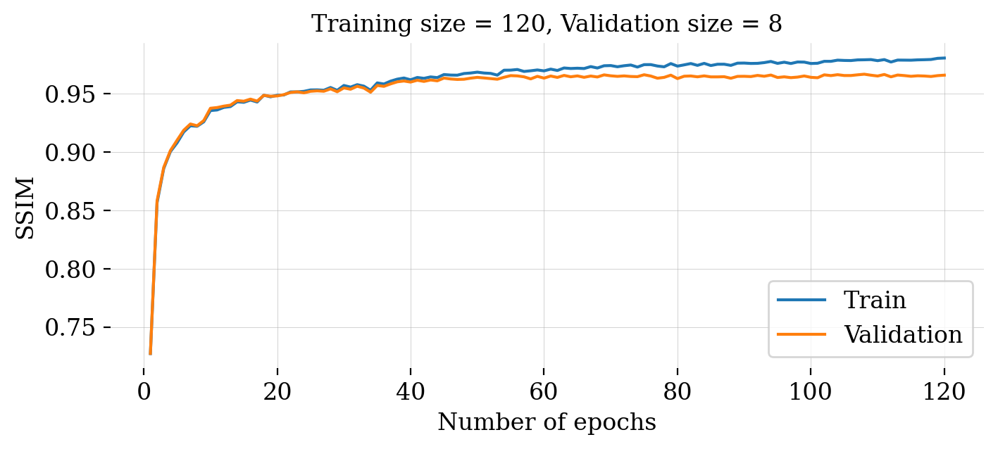
Given the \(\textsc{Forecast}\) ensemble, \(\{\mathbf{x}_k^{(m)},\mathbf{y}_k^{(m)}\}_{m=1}^{M}\), the subsequent step is to compute the optimized training weights, \(\widehat{\boldsymbol{\phi}}_k\). After random initialization, the network weights are trained by minimizing the objective on line 9 of Algorithm 2 with the optimizer \(\textsc{ADAM}\) (Diederik P. Kingma and Ba 2014) and for a total of \(120\) epochs. As we can see from figure 8, the plots for the \(\ell_2\)-norm training objective and SSIM (see Appendix B) both behave as expected during training and validation and there is no sign of overfitting.
To measure the performance of our network, we also plotted the structural similarity index measure (SSIM, Z. Wang et al. (2004b)), which is a metric designed to mimic human perception of image quality. See Appendix B for further details.
4.3.3 The Analysis step
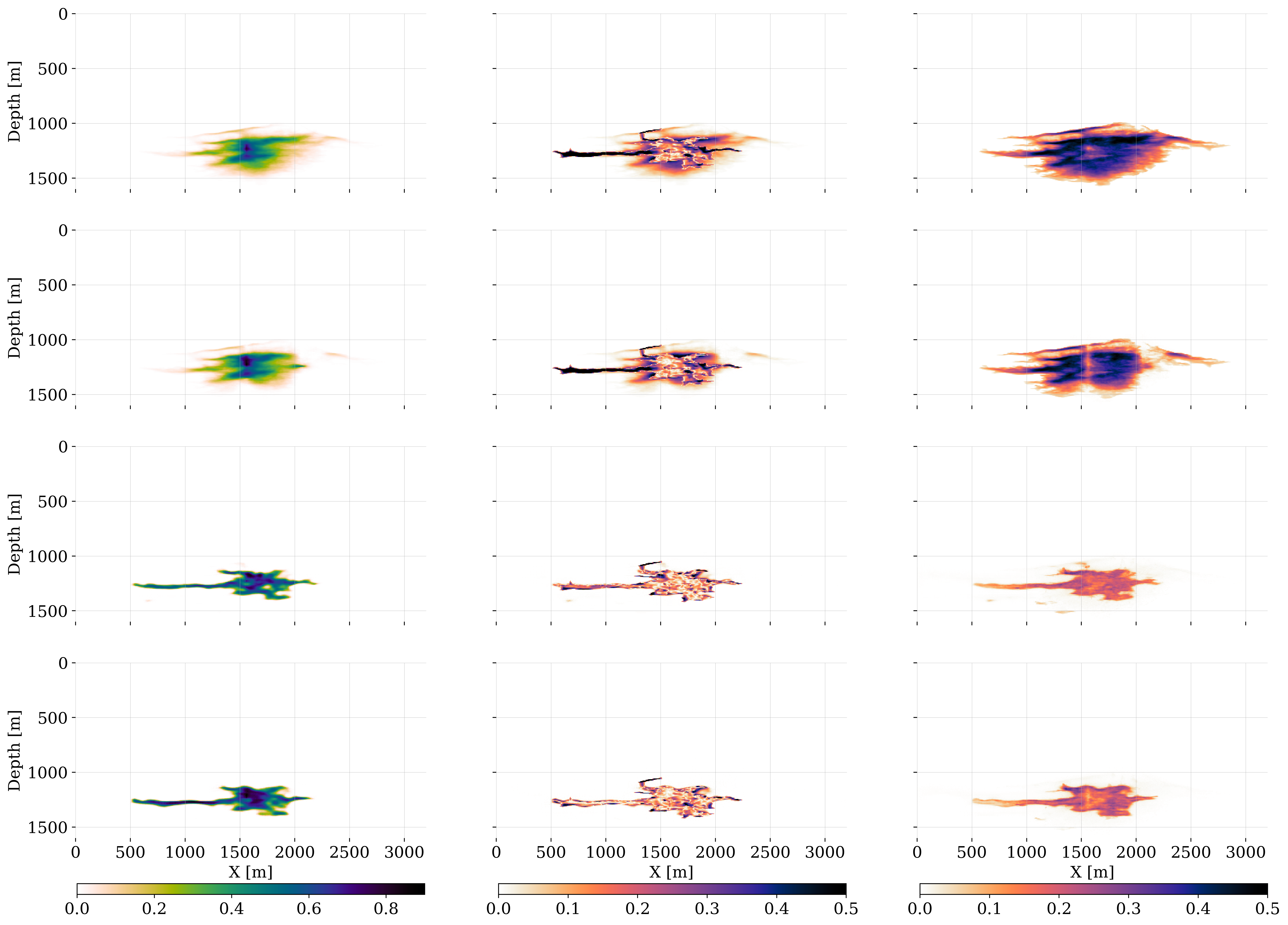
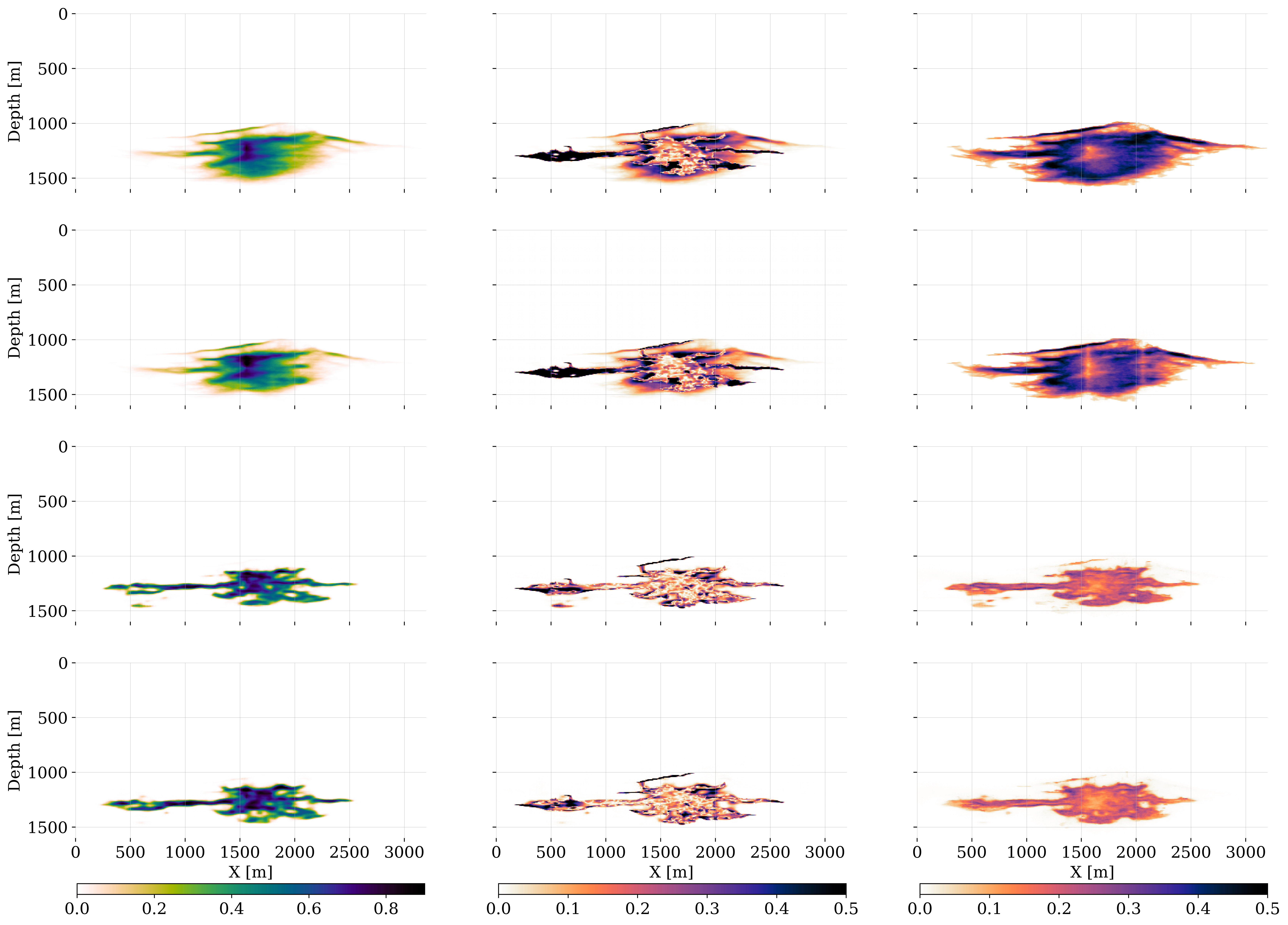
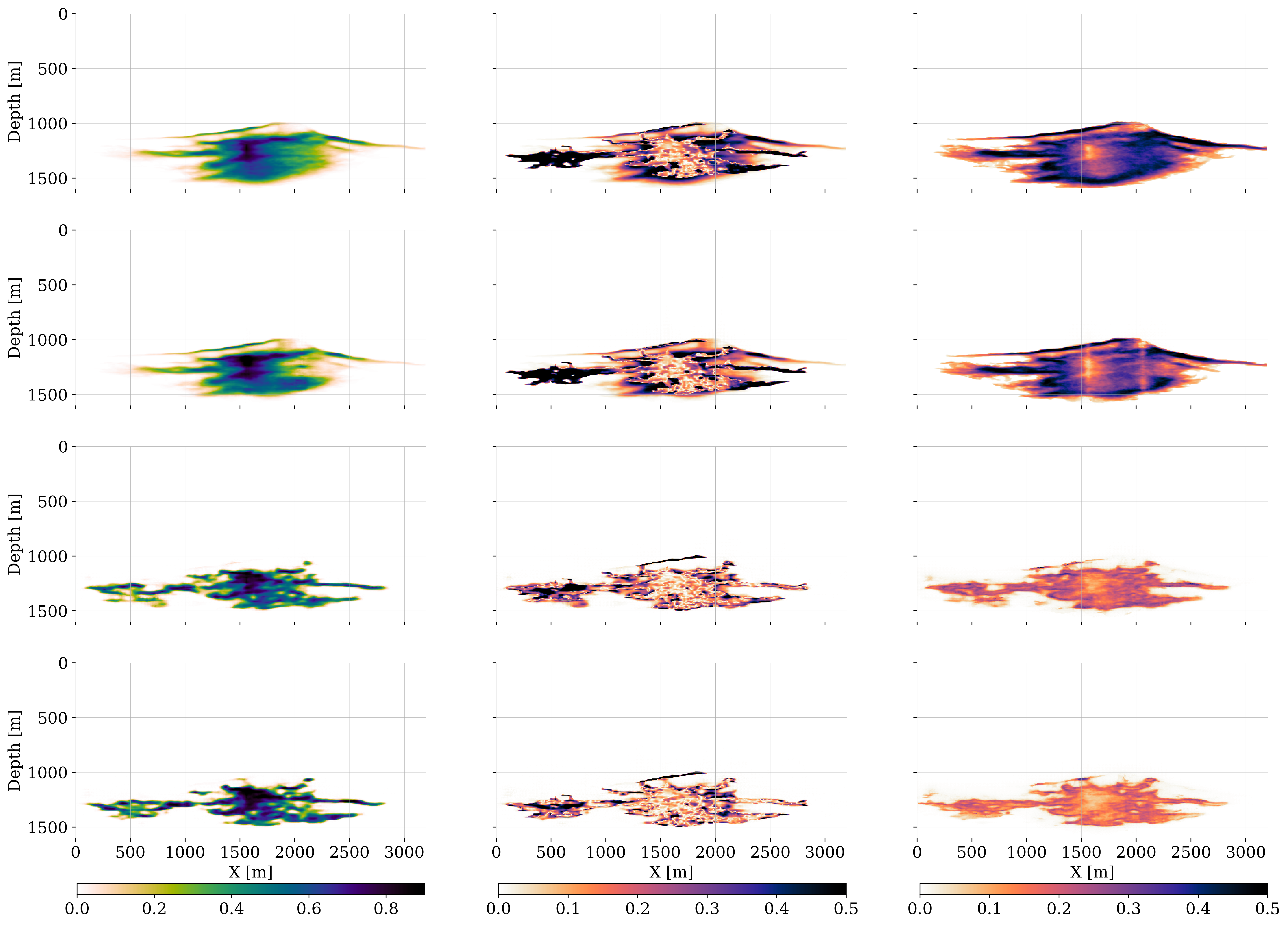
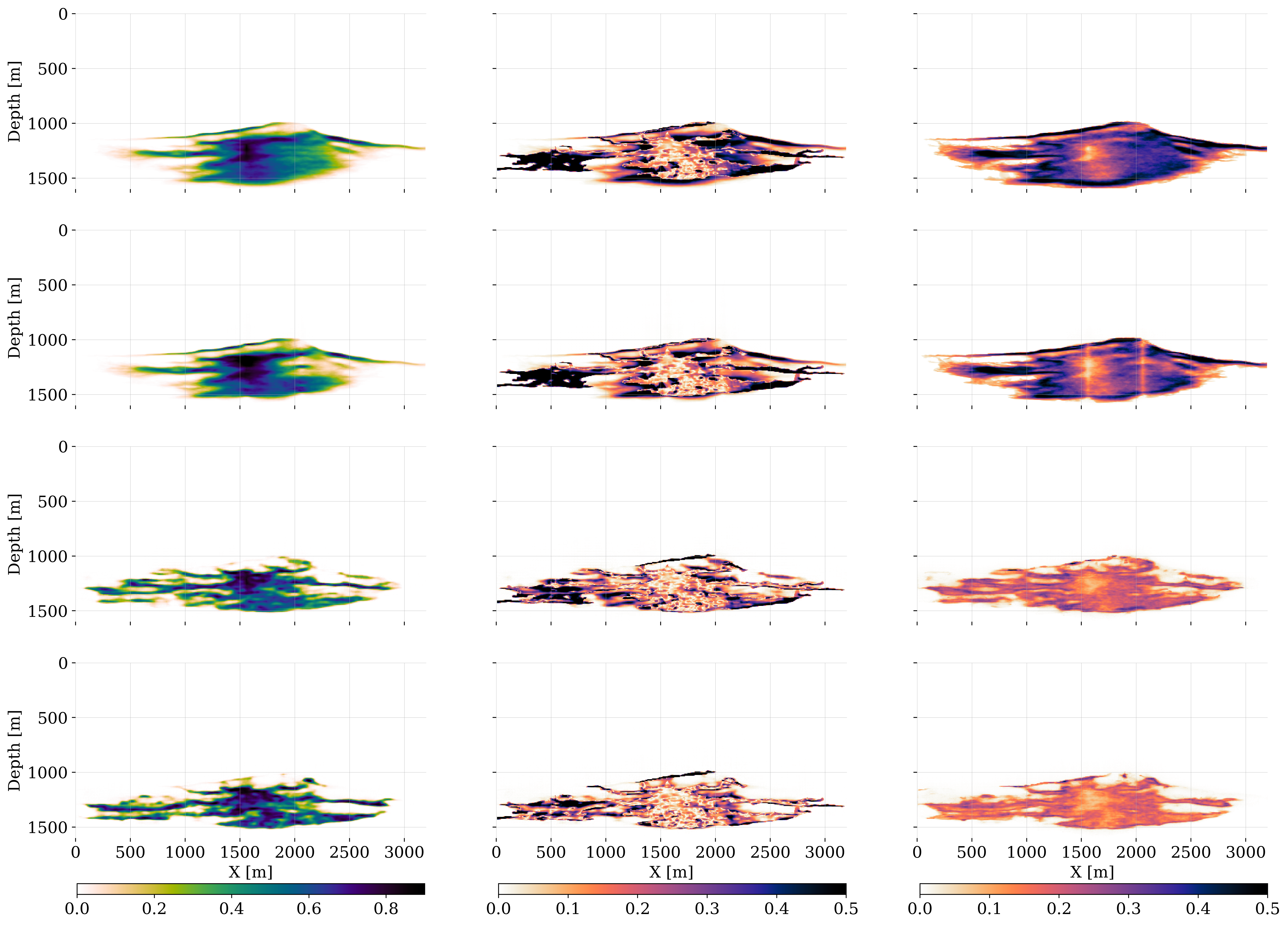
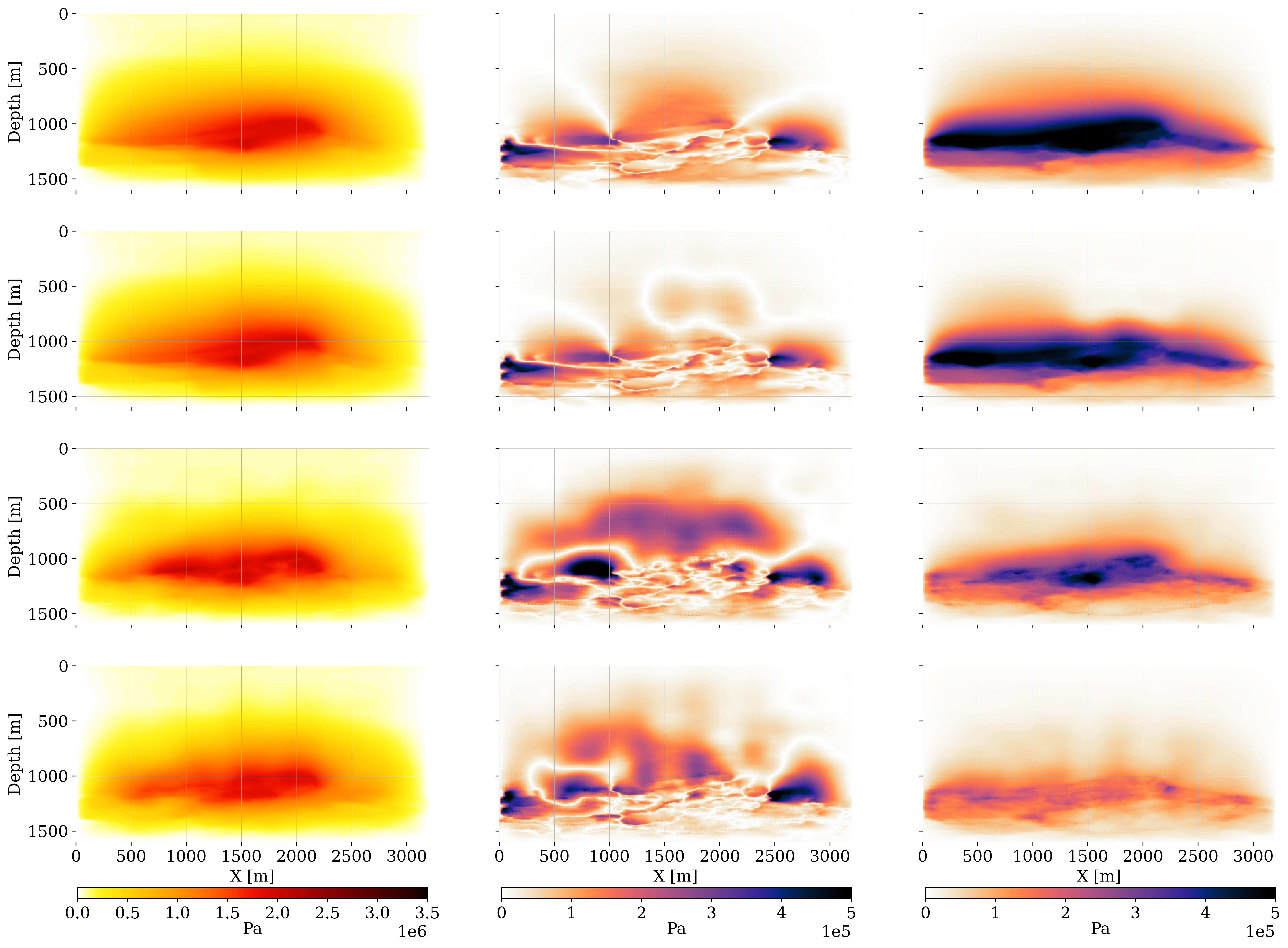
With the networks for the amortized posterior inference trained, the predicted samples in the ensemble for the state, produced by the \(\textsc{Forecast}\) step, are corrected by conditioning the posterior distribution on the imaged “field” data. In our case, the field data consists of the in silico ground-truth simulations outlined in Section 4.2. Given these “time-lapse field datasets”, \(\mathbf{y}_k^{\textrm{obs}}, \, k=1\cdots K\), the predicted states of the ensemble, \(\{\mathbf{x}_k^{(m)}\}_{m=1}^{M}\), are corrected during the \(\textsc{Analysis}\) step, which corresponds to executing lines 14—15 of Algorithm 2 for each timestep, \(k=1\cdots K\). To illustrate the importance of the \(\textsc{Analysis}\) step at timestep, \(k=3\), the first two columns of figure 9 include corrections on a single instance of the predicted state, \(\mathbf{x}_3\sim p(\mathbf{x}_3\mid \widehat{\mathbf{x}}_2)\) with \(\widehat{\mathbf{x}}_2\sim p_{\widehat{\phi}_2}(\cdot\mid \mathbf{y}_2^{\text{obs}})\), and the corrected plume, \(\widehat{\mathbf{x}}_3\sim p_{\widehat{\phi}_3}(\cdot\mid \mathbf{y}_3^{\text{obs}})\). The saturations are plotted in the top row and pressure differences in the bottom row. The correction for the CO2 saturation at timestep, \(k=3\), is smaller than the correction at time step, \(k=1\), as shown in figure 2. The reason for this is that the early correction at the time step, \(k=1\), establishes the leftward fingering feature that persists to the later timesteps. However, this does not apply to the protruding rightward CO2 plume features that come in at later times and which are partially missed by the saturation prediction. While less pronounced, the individual pressure perturbation prediction is also updated considerably during the \(\textsc{Analysis}\) Step.
The impact of the correction also becomes clear from the right-most two columns of figure 9 where the conditional mean before, \(\bar{\mathbf{x}}_3\), and after the corrections, \(\bar{\widehat{\mathbf{x}}}_3\), are juxtaposed. After conditioning on the observed data, the corrected samples exhibit less variation, which results in a significantly better resolved conditional mean for the corrected CO2 saturation. Similarly, the pressure difference corrections yield a pressure field that is more consistent. These improvements during the \(\textsc{Analysis}\) step are also apparent when comparing the errors w.r.t. the ground truth, \(\text{Error}=|\mathbf{x}_3^\ast-\mathbf{\bar{x}}_3|\) vs. \(\text{Error}=|\mathbf{x}_3^\ast-\mathbf{\bar{\widehat{x}}}_3|\), plotted before and after corrections during the \(\textsc{Analysis}\) step in figure 10 for the CO2 saturations (top-row: first two columns). The effect of the correction for the pressure differences (bottom-row: first two columns) is more difficult to interpret. However, the uncertainty in terms of the conditional deviations before, \(\boldsymbol{\bar{\sigma}}_3\), and after the correction, \(\bar{\boldsymbol{\widehat{\sigma}}}_3\), tightens significantly for both the CO2 saturations (top-row: rightmost columns) and pressure differences (bottom row: rightmost columns). The plots for the pressure contain locations of the wells where pressure differences can be measured.
While these results where the \(\textsc{Analysis}\) step reduces the uncertainty are encouraging, we will introduce in the next section a set of quantitative performance metrics before considering a case study where the benefits of working with multimodal will be evaluated.
4.4 Performance metrics
While the main goal of this paper is to present a principled workflow to assess uncertainties in the state of the CO2 plume, another goal of establishing a Digital Shadow for Geological CO2 Storage is to accelerate innovations in monitoring to ensure safe operations towards the regulators and the general public. For this reason, we follow Donoho (2023)’s recipe to set the stage for accelerated development in this field by
releasing all our data under the Creative Commons License. This includes the ground-truth seismic and reservoir models, the creation of the samples for permeability, the generation of the ground-truth state and, “observed” time-lapse data;
making all our code available under the open-source software MIT license. While still work in progress, the aim is to make use of our software as frictionless as possible;
introducing benchmark metrics by which the success of the Digital Shadow is measured quantitatively. The aim is that new methods and proposed improvements to the monitoring life-cycle can quickly be validated in a trusted testbed of benchmarks.
For now, the proposed benchmarks include the methodology presented in this paper. In a later companion paper, comparisons between results obtained by alternative data-assimulation methods will be reviewed.
4.4.1 Benchmark I: reconstruction quality
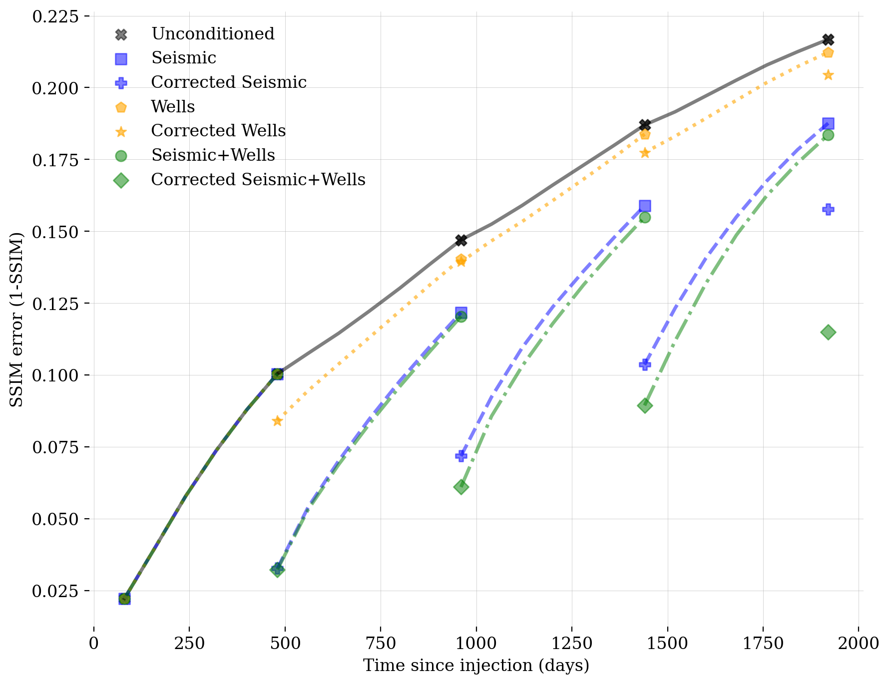
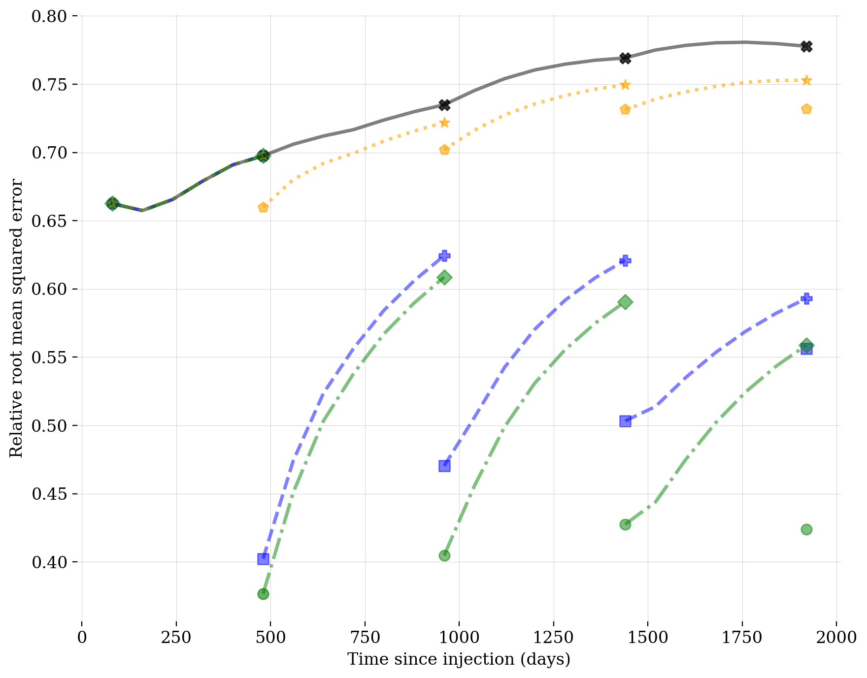
Since the ground-truth state is available as part of our in silico simulations, quantitative assessments of the reconstruction quality can be made by computing the Structural Similarity Index Metric Error (SSIM-ERR) and Root-Mean-Square-Error (RMSE), both detailed in Appendix B.
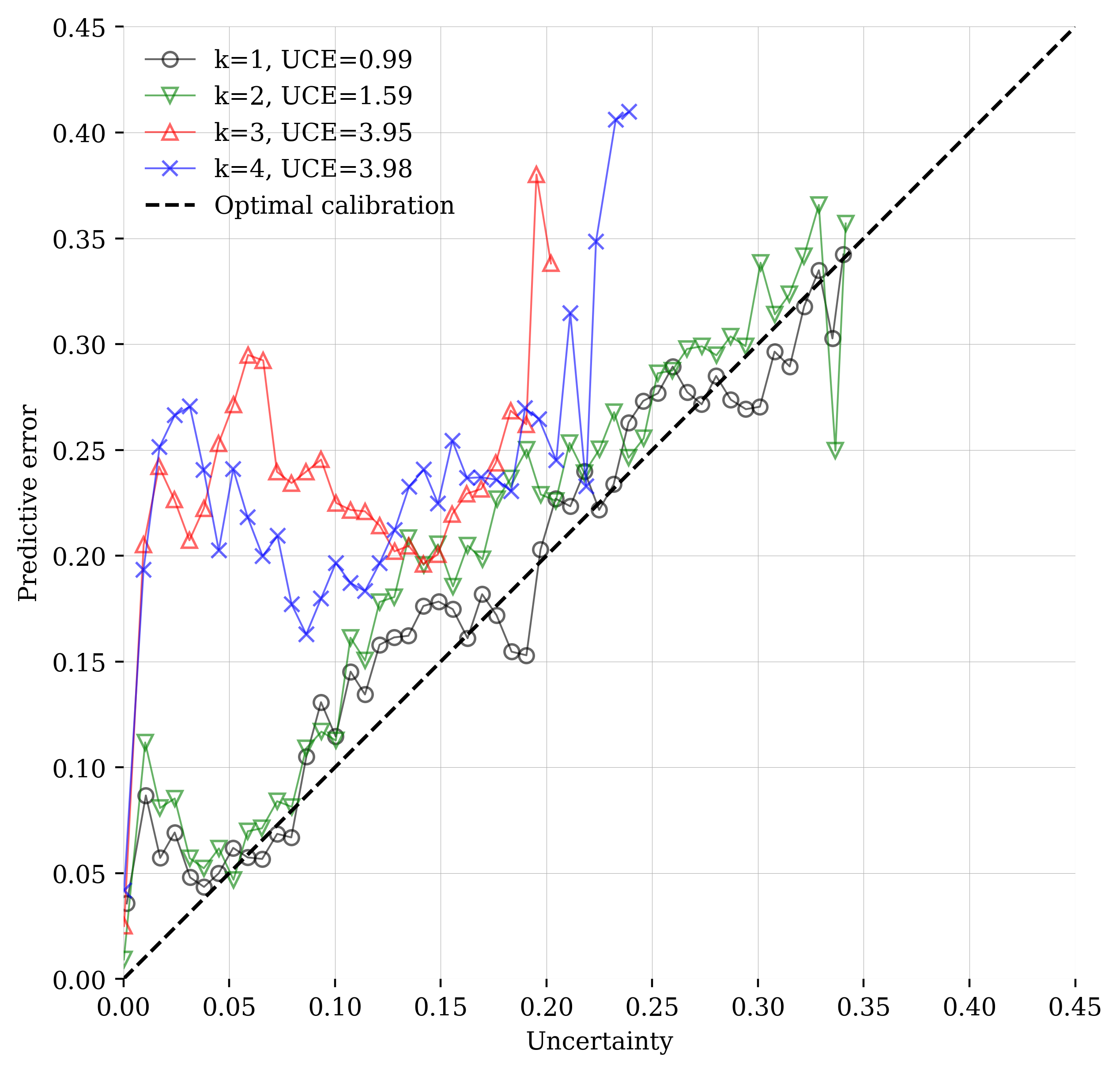
4.4.2 Benchmark II: uncertainty calibration
While the high-dimensionality and computational complexity of our inference problem prevents rigorous validation of the presented statistical analysis, quantitative establishment of how well the predicted uncertainties, \(\widehat{\boldsymbol{\sigma}}_k\), and the errors, \(\text{Error}_k=|\mathbf{x}_k^\ast-\mathbf{\bar{x}}_k|\), correlate is computationally feasible. To this end, we follow Orozco, Siahkoohi, et al. (2024) and introduce the calibration test developed by Guo et al. (2017); Laves et al. (2020). During this test, Euclidean distances are calculated between posterior mean estimates for the state and the ground-truth state. According to this test, uncertainty is well-calibrated when it is proportional to the error. To establish this test, deviations for each gridpoint in \(\widehat{\boldsymbol{\sigma}}\) are designated into \(L\) bins of equal width. The uncertainty for each bin, \(B_l\), is then calculated with
\[ \mathrm{UQ}(B_l) = \frac{1}{|B_l|} \sum_{i\in B_l}\bar{\boldsymbol{\widehat{\sigma}}}[i] \]
where \(\bar{\boldsymbol{\widehat{\sigma}}}[i]\) refers to the \(i^{\text{th}}\) entry of the estimated deviation vector. For each bin, the mean-square error w.r.t. the ground truth is calculated with
\[ \mathrm{MSE}(B_l) = \frac{1}{|B_l|} \sum_{i\in B_l}(\mathbf{x}^{\ast}[i] - \widehat{\mathbf{x}}[i])^2. \]
Qualitatively, good uncertainty calibration implies that points on the crossplot between the predicted error and actual uncertainty fall along the line \(y=x\). To quantify the quality of uncertainty calibration, we follow Orozco, Siahkoohi, et al. (2024) and calculate the Uncertainty Calibration Error (UCE), defined as the average absolute difference between the predicted error and actual uncertainty across all bins. A lower UCE indicates more precise calibration, which is approximately the case in figure 11 for the posterior samples conditioned on both seismic and wells. We observe a trend towards poorer calibration as the monitoring time step increases. We hypothesize that as the plume grows larger, there are more areas where errors can occur, making the calibration test more difficult to pass. When comparing a new method under this benchmark, we would qualitatively evaluate the calibration plots on a per-monitoring time basis, and also in aggregate, to summarize performance across all monitoring times. As a quantitative metric, we would compare the UCE values between methods and select the one with the lowest UCE as having the best calibration.
5 Multimodal case study
The task of the proposed Digital Shadow is to produce high-fidelity estimates for the state of the CO2 plume using a combination of data-assimilation and machine learning techniques that use multimodal time-lapse data as input. Aside from conducting principled uncertainty quantification, the aim is also to maximally benefit from having access to two complementary time-lapse datasets, namely time-lapse pressure/saturation measurements at the two wells (injection and monitoring) and 2D active-source time-lapse seismic surveys. The aim of these in silico experiments is to demonstrate the possible benefits of multimodal data-assimilation over data comprised of well or seismic data only. To this end, inferences will be carried out on both time-lapse datasets separately and jointly. After briefly describing the relative ease by which the presented Digital Shadow can be extended to include data collected at (monitoring) well(s), systematic quantitative comparisons will be made between the different approaches. This includes quantitative analyses based on the metrics introduced in Section 4.4.
5.1 Data collection, simulation, and training
While inverting multimodal data in classical (read without machine learning) inversion/inference problems has proven challenging, especially when the different datasets are scaled differently, or collected differently, extending the proposed neural data-assimilation framework is relatively straightforward as long as the time-lapse data are collected on the same grid and at the same discrete observation times. Under that assumption, observations of the saturation/pressure (\(\mathbf{x}_k[S_{\mathrm{CO_2}}]\) and \(\mathbf{x}_k[\delta p]\)) data can be modeled by a restriction operator, collecting these quantities at gridpoints that correspond to the well locations. During training and inference, time-lapse saturation, pressure, and seismic images each serve as input to separate input channels of the conditional branch of the cINN. The saturation and pressure are both converted to all-zero images except for values of the saturation and pressure at the well locations. Based on conditioning, by seismic only, well only, or both, the cINN is trained to produce samples of the state, consisting of gridded images for saturation and pressure perturbation. These gridded quantities are produced by separate output channels of the network. The experiment setup for the ground truth and is the same as outlined in Section 4.
5.2 Experimental protocol
Experiments to investigate the possible benefits of multimodal acquisition proceed as follows:
Initialization step: Draw \(M=128\) samples from the initial distribution for the state, \(\widehat{\mathbf{x}}_0\sim p(\mathbf{x}_0)\). The initial saturation is selected from the uniform distribution on the interval \([0.1,\, 0.6]\) and chosen to occupy a cylinder with a diameter of four grid cells (\(4\times 6.25\mathrm{m}\)). The location of the cylinder coincides with the injection interval at the well, which extends \(37.5\mathrm{m}\), vertically. The vertical location of the well’s injection interval is positioned adaptively within the closest high-permeability layer in the randomly drawn permeability fields, \(\boldsymbol{\kappa}\sim p(\boldsymbol{\kappa})\). These permeability fields are drawn with replacement from a set of \(1000\) converted velocity models produced by WISE. The resulting injection depth varies between \(1200-1250\mathrm{m}\). The initial pressure is set to the hydraulic pressure, which increases with depth. This initialization produces the initial ensemble for the state, \(\{\widehat{\mathbf{x}}_0^{(m)}\}_{m=1}^{128}\).
Forecast step: For each timestep, the state and multimodal observations are predicted by time advancing the state ensemble, \(\{\widehat{\mathbf{x}}_{k-1}^{(m)}\}_{m=1}^{128}\), to \(\{\mathbf{x}_k^{(m)}\}_{m=1}^{128}\) by running the dynamics (cf. equation 1), followed by sampling from the “likelihood” (cf. equations 2, 14, 15). This produces the predicted ensemble, \(\{(\mathbf{x}_k^{(m)}, \mathbf{y}_k^{(m)})\}_{m=1}^{128}\). These predicted states consist of the saturation, \(S_{CO_2}\), and pressure perturbation, \(\delta\mathbf{p}\), with respect to the initial hydraulic pressure. Depending on the time-lapse data modality, the simulated observations, \(\{\mathbf{y}_k^{(m)}\}_{m=1}^{128}\), consist of imaged seismic, saturation/pressure, or both.
Training step: The predicted ensembles, \(\{\mathbf{x}_k^{(m)}\}_{m=1}^{128}\), are split into \(120\) training samples and eight validation samples. After the network training is completed, the inference is carried out on one sample of the test set, which consists of the ground-truth seismic images, \(\mathbf{y}_k^{\mathrm{obs}}\).
Analyses step: Conditioned on observed time-lapse “field” data, \(\mathbf{y}^{\mathrm{obs}}_k\), the predicted states are corrected by computing the latent representation for each ensemble pair, followed by sampling from the posterior conditioned on the field observations by running the cINN in reverse on the latent variables (cf. equations 12 and 13). This produces the corrected ensemble for the states, \(\{\widehat{\mathbf{x}}_{k}^{(m)}\}_{m=1}^{128}\).
By applying the \(\textsc{Forecast}\) and \(\textsc{Analysis}\) steps recursively, the full history of the estimated state for each member of the ensemble is collected in the vectors \(\{\widehat{\mathbf{x}}_{1:24}^{(m)}\}_{m=1}^{128}\). These complete state histories are formed by appending six dynamic simulation timesteps after each member of the ensemble is corrected during the \(\textsc{Analysis}\) step. Given these complete histories for the state, we proceed by calculating point estimates, in terms of the conditional mean, \(\bar{\widehat{\mathbf{x}}}_{1:24}\) and their uncertainty in terms of the conditional deviations, \(\bar{\widehat{\boldsymbol{\sigma}}}_{1:24}\), for all \(24\) timesteps. To quantify the data-assimilation accuracy of the inferred states, the errors with respect to the ground truth, \(\mathbf{e}_{1:24}=|\mathbf{x}^\ast_{1:24}-\mathbf{\bar{\widehat{x}}}_{1:24}|\), will be calculated as well.
5.3 Qualitative results
To establish the performance of the proposed Digital Shadow, juxtapositions are made between data-assimilations for three different data modalities, namely well only, seismic only, and well + seismic. The importance of data-assimilation compared to relying on reservoir simulations alone will also be demonstrated by comparing plots for the conditional mean (\(\bar{\widehat{\mathbf{x}}}_{1:6:24}\)), the errors with respect to the ground truth, \(\mathbf{e}_{1:6:24}=|\mathbf{x}^\ast_{1:6:24}-\mathbf{\bar{\widehat{x}}}_{1:6:24}|\), and the conditional standard deviation, \(\bar{\widehat{\boldsymbol{\sigma}}}_{1:6:24}\) for these three different modalities. These quantities are calculated from posterior samples, conditioned on the simulated ground-truth time-lapse data included in figure 12 for \(k=1\cdots 4\). This figure contains plots for the ground-truth saturation, \(\mathbf{x}^\ast_k[S_{\mathrm{CO_2}}]\); pressure perturbations, \(\mathbf{x}^\ast_k[\delta p]\), including locations of the wells, and plots for the corresponding noisy imaged seismic observations in the third column. Observations at wells and/or imaged surface seismic are collected in the vectors, \(\mathbf{y}^{\mathrm{obs}}_k\), for \(k=1\cdots 4\), and serve as input to our Digital Shadow whose task is to infer the state of the CO2 plume for each timestep.
Estimates for the CO2 saturation states \(\bar{\widehat{\mathbf{x}}}_{1:6:24}\), \(\mathbf{e}_{1:6:24}=|\mathbf{x}^\ast_{1:6:24}-\mathbf{\bar{\widehat{x}}}_{1:6:24}|\), and \(\bar{\widehat{\boldsymbol{\sigma}}}_{1:6:24}\) are, for each of the four scenarios (unconditioned, conditioned on well only, seismic only, well + seismic) included in the rows of figures 13—16 for \(k=1\cdots 4\). The corresponding estimates for the pressure perturbations \(\mathbf{x}_{1:6:24}[\delta p]\) are shown in Appendix B. The columns of these figures contain estimates for the conditional mean, errors, and uncertainty in terms of the standard deviation. From these plots, the following qualitative observations can be made.
First, and foremost, a comparison between the unconditioned and conditioned CO2 plume estimates shows that conditioning on any type of time-lapse data nudges, for each timestep, the corrected fluid-flow predictions closer to the ground-truth CO2 saturations. As expected, the unconditioned CO2 plume diverges due to epistemic uncertainties induced by the unknown permeability field at each time-lapse timestep (\(k=1\cdots 4\)). Remember, every time the dynamic state equation (cf. equation 1) is run, a new sample for the permeability field is drawn, introducing new uncertainties into the system. This effect is also present for the CO2 plume estimates conditioned on time-lapse data but to a much lesser degree because the insertion of time-lapse data cancels some of the systematic uncertainty. However, including time-lapse data at the wells by itself does not move the overall shape of the inferred CO2 plume much closer to the ground truth. Nevertheless, when the conditioning involves seismic data, the corrections capture the overall shape of the CO2 saturations very well.
Second, the conditional mean estimates for the CO2 saturation appear smooth compared to the ground truth. This smoothing effect is due to the remaining uncertainty of the estimated plumes (see column three of figures 13—16) and persists, and even increases somewhat, as time progresses.
Third, the CO2 plume estimates at \(k=1\) obtained for the wells only completely miss the important leftward protruding CO2-plume feature, which eventually leads to a violation of Containment. Conversely, this feature is well recovered by inferences based on time-lapse data that includes imaged seismic. Compared to seismic only, joint inference from well + seismic data shows further improvements near the wells and away from the wells, reducing the error with respect to the ground-truth CO2 saturation (see column two of figures 13—16). As expected, including pressure and saturation data at the wells reduces uncertainty in the direct vicinity of the wells but there are also indications that it may have an effect away from the wells when combined with time-lapse seismic. Finally, the errors and uncertainty in terms of the conditional standard deviations correlate reasonably well when the CO2 plume is conditioned on both time-lapse seismic and well data.
Fourth, the overall trend continues at timestep, \(k=2\), leading to reduced errors and uncertainty in the main body of the plume when the CO2-plume inference is conditioned on well + seismic data. However, because of a lack of lateral information the results based on well data alone more or less completely miss the important leftward-protruding streamline feature induced by the unknown high-permeability streak.
Fifth, the complexity of the CO2 plume increases further at later timesteps. This challenges the inference. However, we note again that the estimated conditional mean improves considerably when the inference is conditioned on time-lapse seismic data. As can be observed in figure 15 and 15 bottom first and third column, the inference improves due to the inclusion of information at the wells. As a result, uncertainty is reduced in regions away from the wells both horizontally, and vertically below the wellhead. Interestingly, while the well-only inference result lacks detail, its uncertainty at the horizontal extremities seems to suggest protruding fingers at the periphery of the CO2 plume. These features are indeed present in the ground-truth CO2 plume and in the inferences that include time-lapse seismic data.
Sixth, the conditional mean estimates for the CO2 plume are for most features best recovered when the inference is conditioned on time-lapse seismic data with visible improvements when pressure and saturation data collected at the wells are included. When comparing the uncertainty (column three of figures 13—16), it appears that adding pressure/saturation data from the wells also reduces the uncertainty in areas relatively far away from the well-bore. Finally, the well-only inference seems to include increased CO2 saturation at the seal, a feature that is only partly present in the ground truth. The presence of this feature can attribute to the average behavior of the permeability, an observation shared by the unconditioned results. It is encouraging to see that this feature at the seal has large uncertainty judged by the large \(\bar{\widehat{\boldsymbol{\sigma}}}_{24}\) in this region. Except for an area near the well-bore, CO2-plume saturations are not visible on the conditional mean estimates conditioned on the seismic. However, there is a small imprint on the plots for the uncertainty, which means that the posterior samples do include sporadic examples of detectable CO2 saturation in this narrow area near the seal.
While these inference results by the Digital Shadow are encouraging, they only provide snapshots at the four timesteps time-lapse data is collected. They also do not provide quantitative information on the performance of the proposed Digital Shadow.
5.4 Quantitative results
Since the inference results produced by the Digital Shadow will be used during decision making by a Digital Twin, a better understanding needs to be gained on the performance of the Digital Shadow by means of a quantitative analysis of the different inference strategies. To this end, we include in figure 17 calculations of the SSIM-ERR defined as \(1-\mathrm{SSIM}(\cdot)\), the mean absolute error (MAE), and the mean standard deviation (\(\bar{\sigma}_k\)), for all \(24\) timesteps spanning a total of \(1920\) days. To compensate for biases induced by the growth of the CO2 plumes themselves, the following relative measures will be used for the errors and standard deviations:
\[ \Delta\mathrm{RMSE}_k(\widehat{\mathbf{x}}_k) = \frac{\mathrm{RMS}(\mathbf{e}_k)}{\mathrm{RMS}(\mathbf{x}^\ast_k)}\quad \text{and}\quad \Delta\mathrm{STD}_k=\frac{\mathrm{mean}(\bar{\mathbf{\widehat{\boldsymbol{\sigma}}}}_k)}{\mathrm{RMS}(\widehat{\mathbf{\bar{x}}}_k)} \tag{22}\]
where \(\mathrm{RMS}\) stands for Root-Mean Square. The normalization of the \(\mathrm{RMS}\) for the error and the mean standard deviation by the \(\mathrm{RMS}\) of the ground truth and estimated conditional mean is meant to correct for increased variability exhibited by growing CO2 plumes.
Each subplot in figure 17 contains estimates for these quantities based on inferences conditioned on seismic only (dashed blue lines), on wells only (dotted orange lines), and seismic + wells (dashed-dotted green lines). To exemplify the importance of conditioning fluid-flow simulations on time-lapse observations, we also plot estimates obtained without conditioning (solid black lines) obtained by running equation 1 recursively for \(k=1\cdots 4\). From these three plots, the following observations can be made.
First, the curves for the SSIM-Error, \(\Delta\mathrm{RMSE}_k\), and \(\Delta\mathrm{STD}_k\) overall show improved quality in all three metrics when constrained by time-lapse observations (all other than black curves). Moreover, significant enhancements as a result of the \(\textsc{Analysis}\) step can be observed thanks to time-lapse data-informed corrections on the predictions of the \(\textsc{Forecast}\) step. These corrections start by being relatively small when conditioning on the well measurements alone (cf. the orange star (corrected) and pentagon symbols) but become more significant when conditioning on the seismic (cf. the blue cross and square symbols) and even more pronounced when conditioning on well + seismic (cf. green diamond and round symbols). As time evolves, the magnitude of the data-informed corrections increases for all metrics with the largest improvement in \(\mathrm{SSIM-Err}\) at the last timestep, which can be explained because the bulk of the CO2 plume will have reached the monitor well at that time. Since the state dynamics and observation model are both nonlinear, this significant improvement can not be explained by the corrections from the well data alone.
Second, for each timestep in between the time-lapse data collection, there is, as expected, a general downward trend in plume recovery quality from the time the corrections are made until the next timestep during which the next time-lapse data is collected and the subsequent corrections are made. This deterioration in recovery quality is observed for the \(\mathrm{SSIM-Err}\) for all modalities and is to leading order the result of differences between the randomly drawn permeability field and the ground truth that lead during the intermediate timesteps to increasing deviations between the actual CO2 plume and the predicted ensemble produced by the \(\textsc{Forecast}\) step. The normalization in the definition of \(\Delta\mathrm{RMSE}_k\) in equation 22 compensates partially for this effect, yielding more prominent improvements, especially between conditioning on seismic data alone or on wells + seismic. In addition, relative errors after correction remain reasonably flat and even decrease at the final timestep. This suggests that relative errors remain more or less constant thanks to the conditioning on multimodal time-lapse observations.
Third, the relative quantity, \(\Delta\mathrm{STD}_k\), aims to answer the question of whether including time-lapse data, and multimodal time-lapse data in particular, reduces the uncertainty. Thanks to the normalization by the \(\mathrm{RMS}\) of the (conditional) mean, the uncertainty plotted in figure 17 (c) remains relatively constant with slightly larger corrections produced by conditioning the CO2 plumes on multimodal time-lapse data. While this behavior is consistent with the behavior displayed by the relative errors in figure 17 (b), the uncertainty measured in terms of the variability amongst the intermediate plume predictions seems to dip further during the immediate timesteps after the corrections are made. This behavior is observed for the unconditioned and conditioned by well-only modalities and can be explained by the fact that after each correction new samples for the permeability distribution field are drawn at which point the flow will first explore regions of high permeability before growing. This explains the observed reduction in variability for the unconditioned and conditioned on well-data-only modalities that produce CO2 plumes that are more widely spread and therefore can explore more regions to fill in. After these regions are filled, the plumes grow again increasing the variability and therefore the uncertainty.
In summary, the overall trends observed in figure 17, are consistent with a highly nonlinear data-assimilation problem where the unknown permeability field that controls the flow is modeled as a random nuisance parameter. Even though there is a slight deterioration in the quality of the inferred CO2 plumes, the observed relative errors and uncertainty remain relatively stable over time when the predicted simulations are conditioned on time-lapse data that includes seismic surveys. While including time-lapse well data alone does not lead to significant improvements in CO2 plume reconstruction quality and uncertainty, combining this data modality with time-lapse seismic data leads to significantly improved results.
6 Discussion
The main goal of this work is the design, implementation, and in sillico validation of a Digital Shadow prototype for Geological Carbon Storage. IBM’s definition of a Digital Twin reads:
A digital twin is a virtual representation of an object or system designed to reflect a physical object accurately. It spans the object’s lifecycle, is updated from real-time data and uses simulation, machine learning and reasoning to help make decisions.
When considering this definition, it is clear that the presented neural data-assimilation framework does indeed capture several key aspects (denoted by italics) of a Digital Twin. Because our formulation does not yet support control, reasoning, and decision-making, we follow Asch (2022) and use the term Digital Shadow for our prototype monitoring framework instead. To help future decision-making and optimize underground CO2 storage operations, we leverage recent breakthroughs in neural posterior-density estimation and generative AI to make our Digital Shadow uncertainty aware, which will help the Digital Twin with future tasks including underground monitoring and control, vital for cost-effective risk mitigation and management.
By taking a neural approach, where the simulated state-observation predictions of the well-established ensemble Kalman filter (EnKF, Asch (2022)) are considered as training samples, we arrive at a formulation where the important \(\textsc{Analysis}\) step no longer relies on empirical estimates for the first- and second-order moments (mean and covariance). Instead, our approach hinges on generative conditional neural networks’ ability to characterize non-Gaussian posterior distributions with high degrees of freedom. These distributions result from nonlinear models for the state dynamics (multi-phase flow) and observations (e.g. seismic images), which contain probabilistic components that give rise to complex uncertainties. Compared to other ensemble-based data-assimilation methods (Frei and Künsch 2013), which are typically contingent on Monte-Carlo approximations of the classical Kalman recursions together with limiting Gaussian assumptions, our nonlinear extension of the EnKF enjoys certain important advantages. Backed by the recent work of Spantini, Baptista, and Marzouk (2022), there are strong indications that our approach does not suffer from an unresolvable lack of accuracy of EnKF whose accuracy can not be improved by increasing the ensemble size. Similar to Spantini, Baptista, and Marzouk (2022), we identify corrections during the stochastic prior-to-posterior map as a Kalman-like \(\textsc{Analysis}\) step, implemented in the Gaussianized latent space of a conditional Invertible Neural Network (cINN, Ardizzone et al. (2019b)). Compared to existing ensemble-based methods, the use of conditional neural networks has the advantage that their accuracy, and hence the latent-space correction, increases when adding computational training effort, e.g. by growing the ensemble size or by training with more epochs. When the network is adequately expressive, these accuracy improvements are likely when the set of simulated training pairs, which correspond to the ensemble, are sufficiently large, diverse, and close in distribution to the actual state and observations.
Throughout each lifecycle, the Digital Shadow trains its networks with Simulation-Based Inference (SBI, Cranmer, Brehmer, and Louppe (2020)) by using nonlinear simulations of the time-advanced state (calculated with equation 1) and associated, possibly multimodal, observations (calculated with equation 2). Because our approach is simulation-based, uncertainties associated with the previous state, the random permeability field, and observational noise are marginalized implicitly (Cranmer, Brehmer, and Louppe 2020). As a result, conditional neural networks act as amortized surrogates for the posterior of the state given (multimodal) observations. Thanks to the marginalization, contributions due to the stochasticity of the permeability distribution and other noise terms are factored into the resulting posterior, which is no longer dependent on this nuisance parameter and on specifics of the noise. Moreover, theoretical connections exist between the EnKF’s \(\textsc{Analysis}\) step and the proposed stochastic latent space prior-to-posterior mapping. Similar to Spantini, Baptista, and Marzouk (2022), this stochastic mapping reads in the latent space of the CNF as follows:
\[ \mathbf{x}_k^{(m)}\mapsto \widehat{\mathbf{x}}_k^{(m)}= f^{-1}_{\widehat{\boldsymbol{\phi}}_k}(\mathbf{z}_k^{(m)};\mathbf{y}_k^{\mathrm{obs}})\quad\text{with}\quad \mathbf{z}_k^{(m)}= f_{\widehat{\boldsymbol{\phi}}_k}(\mathbf{x}_k^{(m)};\mathbf{y}_k^{(m)}). \tag{23}\]
Unlike the EnKF, this correction is nonlinear and corresponds to a transport map where samples from the joint distribution for the state and observations are mapped to the latent space, followed by conditioning on the observed time-lapse data during inversion from the latent space back to the physical state. As reported by Ramgraber et al. (2023), conditioning on the observed data in the latent space can have certain advantages thanks to the Gaussinization of the latent space, a topic which we will further explore in future work. Finally, the use of physics-based summary statistics in our approach to our knowledge also differs from current data-assimilation approaches where dimensionality reduction approaches are more common for the state and not for the observations.
Even though the current implementation of our Digital Shadow is specialized towards multimodal monitoring of Geological Carbon Storage, the presented neural data-assimilation approach is general and ready to be applied to other fields as long as implementations for the offline simulation-based \(\textsc{Forecast}\) step, conditional neural networks, and network training procedure are available to approximate the prior-to-posterior mapping. However, specific choices for the implementation of our Digital Shadow prototype were made contingent on scalability, computational cost, memory footprint, and accuracy of the multi-phase flow and wave simulations. For this reason, our implementation is based on the low-memory footprint Julia implementation for CNFs, InvertibleNetworks.jl (Orozco, Witte, et al. 2024a), in combination with the industry-strength parallel multi-phase fluid-flow simulator, JutulDarcy.jl (Møyner and Bruer 2023), and parallel wave-based Julia Devito Inversion framework inversion package JUDI.jl,(P. A. Witte et al. 2019; Louboutin, Witte, et al. 2023). While our framework allows for other choices, our prototype for the Digital Shadow benefits from the intrinsic parallel capabilities of the fluid-flow and wave simulators and from the fact that the ensemble calculations are embarrasingly parallel. In that respect, the presented scalable approach differs from recent score-based work by (Rozet and Louppe 2023; Bao et al. 2024; X. Huang, Wang, and Alkhalifah 2024), which either rely on many, and therefore fast evaluations of the dynamics and observation operators, or on fast access to the complete history of the CO2 plume’s dynamics, neither of which are conducive to realistic scale data-assimilation for GCS projects.
Because of the relatively long lead time between the collection of time-lapse seismic surveys, we so far did not opt for the use of our parallel implementation of Fourier Neural Operators (FNO, Grady et al. (2023)), which in principle can serve as a suitable substitute to the expensive multi-phase flow simulations (Louboutin, Yin, et al. 2023; Yin, Orozco, et al. 2023). We also reserve inclusion of geomechanical, chemical, and (poro-) elastic effects, to future research even though these effects can in principle be included in the Digital Shadow’s simulations. These extensions would allow for the use of our Digital Shadow in more complex situations, including GCS on land, where geomechanics could play a more important role, or within reservoirs that undergo geochemical changes.
Compared to contemporary approaches to CO2 monitoring (C. Huang and Zhu 2020; Grana, Liu, and Ayani 2020), the proposed Digital Shadow’s conditional neural networks are capable of capturing the nonlinear state dynamics, given by the multi-phase flow, and nonlinear seismic observation model, involving nonlinear solutions of the wave equation. Our current implementation achieves this at a scale where extended Kalman filters struggle to store explicit matrix representations for the Kalman filter that includes explicit inverses of large matrices. Like recent work by Bruer et al. (2024), the proposed approach reaps information from an ensemble of states, which is an approach that scales well. By treating the permeability field as a stochastic nuisance parameter, which is drawn independently at each time-lapse timestep for each ensemble member, our Digital Shadow distinguishes itself from this latest work on an EnKF for GCS where the randomly drawn permeability field remains fixed within each member of the ensemble. Aside from incorporating stochasticity induced by the unknown permeable field, which can be interpreted as a modeling error connecting this work to Si and Chen (2024), our approach is also based on a nonlinear seismic observation model.
Finally, the presented approach made assumptions on the distribution of the permeability field as well as on the underlying rock and wave physics. In future work, we will relax these assumptions by (i) extending recent work by Yin, Louboutin, et al. (2024) to carry out permeability inference from time-lapse seismic and/or well data, which would allow for narrowing of the baseline probability distribution for the permeability field, as time-lapse data becomes available; (ii) marginalizing over uncertainties in the rock-physics model, e.g. by augmenting the Forecast ensemble with samples generated from models other than the patchy saturation model (Avseth, Mukerji, and Mavko 2010); (iii) calibrating rock-physical relations at (monitoring) wells (Feng et al. 2022); (iv) robustifying the inference with respect to distribution shifts either through physics-based latent-space corrections, as proposed by Yin, Orozco, and Herrmann (2024) and Orozco, Siahkoohi, et al. (2024), or by adapting score-based methods to solve the weak formulation proposed by Siahkoohi, Rizzuti, and Herrmann (2020) and Orozco, Siahkoohi, et al. (2024); (iv) no longer insisting on costly seismic survey replication to achieve repeatability of time-lapse seismic surveys (Oghenekohwo et al. 2017; Wason, Oghenekohwo, and Herrmann 2017; López et al. 2023; Y. Zhang et al. 2023) (v) increasing detectibility of time-lapse changes in the density by using SH-polarized shear waves (Clochard et al. 2018).
7 Conclusions
The inherent high degrees of freedom and complications arising from the intricate interplay between the nonlinear multi-phase flow, nonlinear rock physics, and possibly nonlinear multimodal time-lapse observations, challenge the development of monitoring systems for subsurface storage of supercritical CO2. In this work, we meet these challenges by introducing an uncertainty-aware Digital Shadow, which combines state-of-the-art high-fidelity simulation capabilities with data-assimilation and machine-learning techniques to arrive at a scalable formulation that through the deployment of a stochastic nuisance parameter incorporates nonlinearities and inherent uncertainties in the permeability field. Thanks to the Digital Shadow’s use of simulation-based inference, its neural networks marginalize over this stochastic permeability field, factoring lack of knowledge on this important reservoir property into Digital Shadows’ uncertainty quantification. As a result, dependence on the permeability field is eliminated and its uncertainty is absorbed into the recursively inferred posterior distributions for the CO2 plume’s state (pressure/saturation), conditioned at each timestep on multimodal time-lapse measurements. The training itself takes place recurrently on \(\textsc{Forecast}\) ensembles, consisting of predictions for the state and simulations of induced time-lapse data collected at the surface and/or in wells.
To validate the proposed Digital Shadow, a realistic simulation-based case study was conducted, starting from a probabilistic model for the permeability field derived from a baseline surface seismic survey. Next, the Digital Shadow’s network was trained on \(\textsc{Forecast}\) ensembles, consisting of simulations for the time-advanced CO2 plume’s state and corresponding multimodal time-lapse data. After training was completed, the Digital Shadow’s networks were applied to unseen simulated ground-truth time-lapse data. From this computational case study, the following observations can be made. First, CO2plume estimates based on averages over the \(\textsc{Forecast}\) ensembles behave poorly compared to estimates corrected by observed time-lapse observations. These improvements are achieved irrespective of the permeability field. Second, the crucial imprint of an unknown high-permeability streak was missed when the CO2 plume’s state was conditioned on pressure/saturation measurements at wells alone. Plume inferences conditioned on seismic or seismic and well measurements succeeded in detecting this event that ultimately leads to Containment failure. Third, the inferred pointwise standard deviation amongst the samples of the posterior, which serves as a measure of their uncertainty, correlates well with errors with respect to the ground-truth state. This property persists over the different timesteps and is an indication that the uncertainty quantification is reasonably well calibrated. Fourth, visual as well as quantitative measures of the reconstruction quality show across the board the best results when the CO2 plume’s state is conditioned on both time-lapse seismic and well measurements. While conditioning the CO2 plume on wells only leads to marginal improvements compared to uncorrected forecasts, combination with seismic leads to disproportional improvements even in areas away from the wells. We attribute these global improvements in the inferred state of the CO2 plume to the strong nonlinearity of multi-phase flow. All in all, we argue from this case study that the proposed Digital Shadow tracks the unseen ground-truth physical state accurately for the duration of a realistic CO2injection project. To our knowledge, the proposed methodology constitutes the first proof-of-concept of an uncertainty-aware Digital Shadow that principally encapsulates uncertainty due to unknown reservoir properties and noise present in the observed data. This Digital Shadow will form the basis for a Digital Twin designed to mitigate risks and optimize operations of underground storage projects.
Data and Software Availability
The data underlying the findings of this study and the software developed for it will be made publicly available upon acceptance of the manuscript for publication. Also, full movies of the snapshots shown in the manuscripts will be included during final submission in the online supplementary material.
Acknowledgement
This research was carried out with the support of Georgia Research Alliance and partners of the ML4Seismic Center. This research was also supported in part by the US National Science Foundation grant OAC 2203821.
References
Appendices
Appendix A
Network architecture cINNs
For CNFs, we followed conditional GLOW network architecture (Durk P. Kingma and Dhariwal 2018) implemented in the open-source package InvertibleNetworks.jl (P. Witte et al. 2023). The architecture of Conditional GLOW typically consists of invertible neural network layers, coupled with affine coupling layers, which enable efficient computation of the determinant of the Jacobian matrix. These layers are organized in a hierarchical manner, which offers better expressiveness when compared to the conventional invertible architectures (Dinh, Sohl-Dickstein, and Bengio 2016). This expressivity comes from applying a series of conventional invertible layers (Dinh, Sohl-Dickstein, and Bengio 2016) to the input in a hierarchical manner which results in an invertible architecture exhibiting the potential to depict intricate bijective transformations (Siahkoohi et al. 2023a; Orozco, Witte, et al. 2024b) and hence the ability to learn complex distributions.
Training Setting
| Hyperparameters | Values |
|---|---|
| Batch Size | \(8\) |
| Optimizer | \(\mathrm{Adam}\) (Diederik P. Kingma and Ba 2014) |
| Learning rate (LR) | \(5^{-4}\) |
| No. of training epochs | \(120\) |
| Fixed Noise Magnitude | \(0.005\) |
| No. of training samples | \(120\) |
| No. of validation samples | \(8\) |
| No. of testing samples | \(1\) |
Appendix B
Useful Definitions
After the completion of training, we use the following procedure to calculate the posterior mean:
\[ \mathbf{x}_{\text{pm}} = \mathbb{E}_{\mathbf{x} \sim p(\mathbf{x}|\mathbf{y})} [ \mathbf{x} ] \approx \frac{1}{M} \sum^{M}_{n=1}\mathbf{x}_{\text{gen}}^{i} \text{ where } \mathbf{x}_{\text{gen}}^{i} = f_{\hat{\boldsymbol{\phi}}}^{-1}(\mathbf{z_i};\mathbf{y}) \text{ with } \mathbf{z_i} \sim \mathcal{N}(0,I), \tag{24}\]
where \(\hat{\boldsymbol{\phi}}\) is the minimizer of Equation equation 10.
\(\textbf{SSIM}\) - Structural Similarity Index Metric quantifies the similarity between two images and is commonly used to assess how closely a generated image resembles a ground truth or reference image. It considers image quality aspects such as luminance, contrast, and structure. For the mathematical formulation of SSIM, please refer to the study by (Z. Wang et al. 2004a).
\(\textbf{RMSE}\) - Root mean squared error is used to represent the measure of the difference between ground truth CO\(_2\) saturation image and the posterior mean of the samples generated by the trained network.
Appendix C
\(\textbf{Pressure perturbation}\) - Total reservoir pressure, excluding hydrostatic pressure.
Similar to CO2 saturation states, estimates for the CO2 pressure perturbation, \(\bar{\widehat{\mathbf{x}}}_{1:6:24}[\delta p]\), \(\mathbf{e}_{1:6:24}=|\mathbf{x}^\ast_{1:6:24}[\delta p]-\mathbf{\bar{\widehat{x}}}_{1:6:24}[\delta p]|\), and \(\bar{\widehat{\boldsymbol{\sigma}}}_{1:6:24}\) are, for each of the four scenarios (unconditioned, conditioned on well only, seismic only, well + seismic) included in the rows of figures 18—21 for \(k=1\cdots 4\). The columns of these figures contain estimates for the conditional mean, errors, and uncertainty in terms of the standard deviation. From these plots, the following qualitative observations can be made.
Unlike the CO2 saturation states, the pressure perturbations estimates are relatively smooth similar to the ground truth (cf. figure 12, second column), so the conditional mean estimates (first column of figures 18—21) do not appear to differ substantially amongst the four different scenarios during the four time-lapse time steps. As observed for infered saturations, variations between the posterior samples conditioned on the wells or wells + sesimic (third columns) show reduced uncertainty near the wells. Errors (second colums) with respect to the ground truth do not change much between the different modalities.
Footnotes
To arrive at this acquisition geometry, use was made of reciprocity—i.e., the computational experiments are calculated for \(16\) sources, reducing the computational costs.↩︎
