Time-lapse full-waveform permeability inversion: a feasibility study

Abstract

Time-lapse seismic monitoring necessitates integrated workflows that combine seismic and reservoir modeling to enhance reservoir property estimation. We present a feasibility study of an end-to-end inversion framework that directly inverts for permeability from multiple prestack time-lapse seismic datasets. To assess the method’s robustness, we design experiments focusing on its sensitivity to initial models and potential errors in modeling. Our study leverages the publicly available Compass model to simulate CO₂ storage in saline aquifers. This model is derived from well and seismic data from the North Sea in an area that is currently considered for geological carbon storage.

1 Introduction

Despite significant advancements in reservoir monitoring over recent decades, time-lapse seismic technology continues to face challenges related to cost and efficiency (D. E. Lumley 2001; R. A. Chadwick et al. 2009; A. Chadwick et al. 2010; Furre et al. 2017). Employing 4D seismic workflows, including time-lapse full-waveform inversion (TL-FWI, D. Lumley 2010; Hicks et al. 2016), has become a common practice for estimating changes in the Earth’s elastic properties, facilitating the quantitative interpretation of these changes as indicators of reservoir attributes like fluid content and pressure (Bosch, Mukerji, and Gonzalez 2010; Wei et al. 2017). Recent methodologies aim to leverage time-lapse seismic data for the joint estimation of both elastic and reservoir properties, with a focus on parameters such as saturation and porosity (Bosch et al. 2007; Hu, Grana, and Innanen 2022). However, the integration of seismic imaging workflows with reservoir simulation tools remains limited, constraining the direct application of time-lapse seismic data for permeability estimation directly from multiple time-lapse seismic surveys. A few exceptions exist. For example, Eikrem et al. (2016) uses ensemble Kalman filtering to refine permeability and porosity estimates. Don W. Vasco et al. (2004) and D. W. Vasco et al. (2008) have explored using time-lapse seismic data for linearized inversion to update permeability. Despite these initial attemps, a more systematic and integrated approach for reservoir characterization and monitoring deserves further investigation.

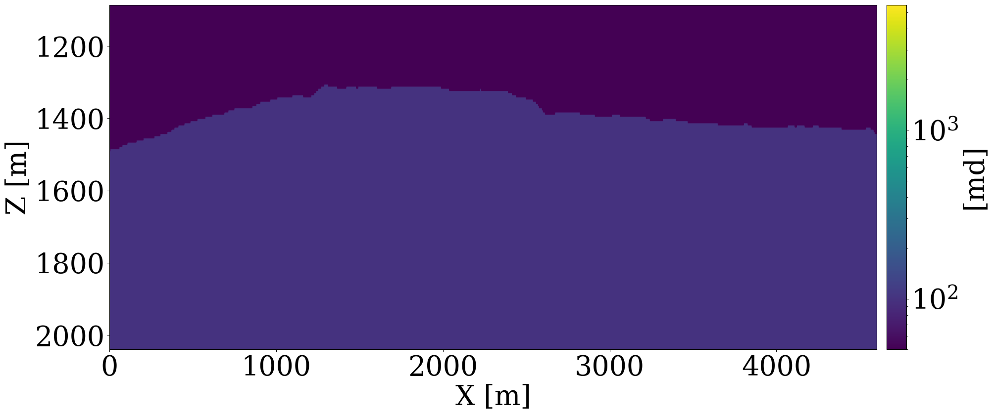
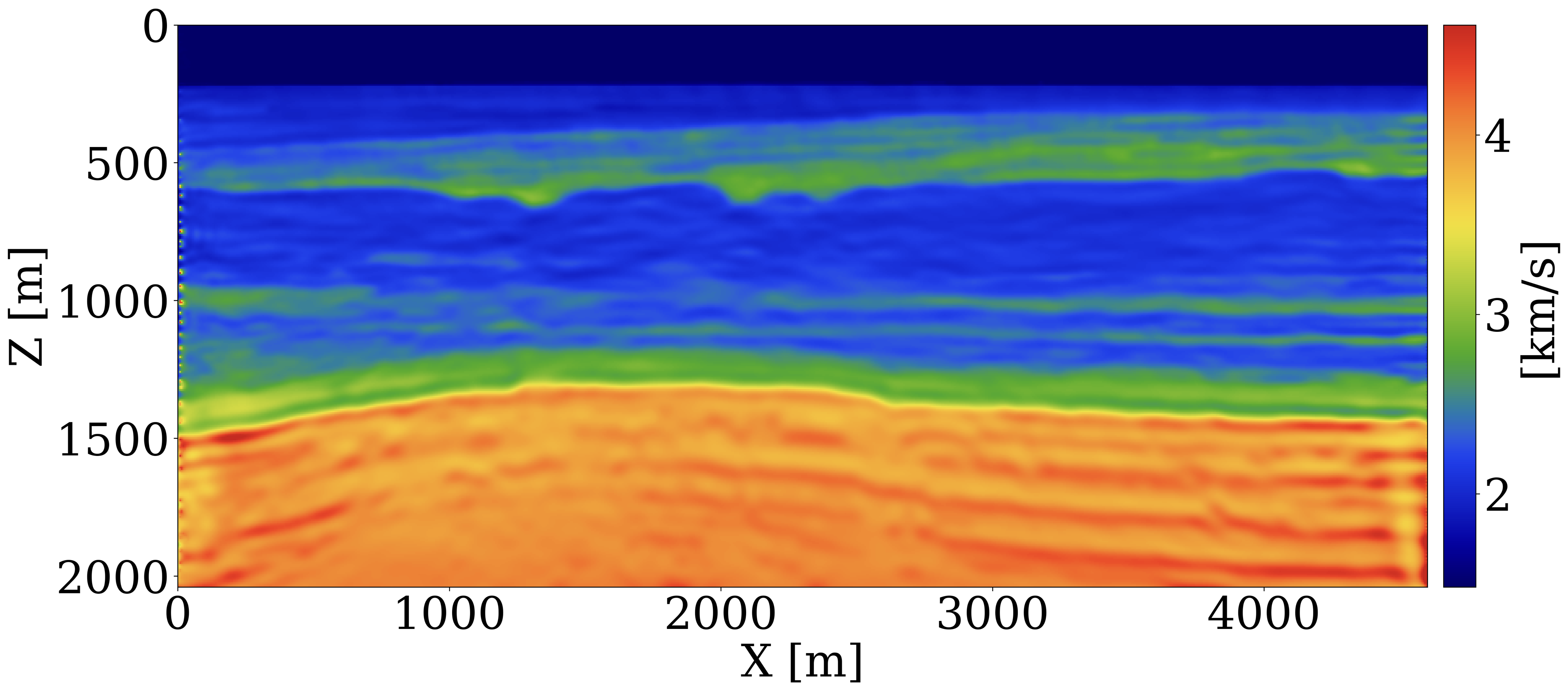
This paper introduces a novel 4D processing framework for estimating permeability directly from prestack time-lapse seismic data, offering a streamlined, geophysics based inversion process. Unlike traditional methods, this framework, tested on various synthetic case studies (Li et al. 2020; Yin et al. 2022; Louboutin, Yin, et al. 2023; Yin, Orozco, et al. 2023), updates permeability models by exclusively matching against multiple observed time-lapse seismic surveys. Despite the potential for rapid model updates, initial results have not yet demonstrated significant alterations in fluid saturation predictions, and the resulting permeability models often lack the heterogeneity necessary for detailed analysis. To address these limitations and to assess the framework’s real-world applicability for 4D monitoring, we undertake a feasibility study using a 2D slice of the Compass model shown in Figure 1. The geological structures of this model were derived from well logs and imaged seismic from the South-West North Sea area — a region under consideration for CO₂ storage (Kolster et al. 2018; Meneguolo et al. 2024). This region comprises a storage unit composed of Bunter sandstone \(300-500 \mathrm{m}\) thick, depicted in orange in Figure 1 (a) and characterized by high permeability values shown in Figure 1 (b). On top of the storage unit there is a primary seal about \(50\,\mathrm{m}\) thick, made of the low-permeable Rot Halite Member, and a secondary seal, over \(300\,\mathrm{m}\), made of low-permeability mudstone in the Haisborough Group, illustrated in blue and green in Figure 1 (a).

(a)

(b)

(c)

Figure 1: Experimental configuration. (a) Setup of seismic acquisition and well control. Dark blue \(\star\) denotes the CO₂ injection well. While \(\times\) and black \(\cdot\) represent source and receiver locations, respectively. The gray curve delineates the shape of the CO₂ plume at the 25th year. (b) Unseen ground truth spatial distribution of horizontal permeability. (c) Histogram of the common logarithm of the permeability model with Kernel Density Estimation (KDE).

This study evaluates the coupled fluid-flow, rock physics, seismic inversion framework’s sensitivity to different starting models, forward modeling errors, and crosstalk during multiparameter inversion, omitting regularization techniques to focus on the impact of time-lapse seismic data on permeability updates. We explore the framework’s ability to recover relatively fine-scale permeability structures, predict CO₂ dynamics within the seismic monitoring period, and forecast CO₂ dynamics in near future without any seismic observation. Recognizing the limitations of our simplifying assumptions, we conclude with suggestions for future research to advance this promising approach.

2 Permeability inversion framework

Our feasibility study examines the time-lapse seismic monitoring of geological carbon storage (GCS), focusing on the integration of three fundamental physics disciplines: fluid-flow physics, rock physics, and wave physics, as illustrated in Figure 2. The dynamics of the CO₂ plume during injection are modeled using multiphase flow equations (Pruess and Nordbotten 2011), processed through a reservoir simulator (Krogstad et al. 2015; Settgast et al. 2018; Rasmussen et al. 2021; Stacey and Williams 2017). While these simulations require detailed inputs, including well operation parameters and the spatial distribution of porosity and permeability, in this exposition we focus on the permeability, \(\mathbf{K}\), particularly, as the parameter of interest. The output from the reservoir simulator, \(\mathcal{S}\), primarily the time-varying CO₂ saturation snapshots, compiled in \(\mathbf{c}\), serves as the input to the rock physics model, \(\mathcal{R}\). Based on the porosity and the brine-filled baseline velocity before CO₂ injection, this model translates each CO₂ saturation snapshot into altered seismic velocity models, compiled in the vector, \(\mathbf{v}\), using the patchy saturation model proposed by Avseth, Mukerji, and Mavko (2010). Lastly, based on the velocity models for each snapshot, the wave modeling operator (Tarantola 1984), \(\mathcal{F}\), is used to generate the time-lapse seismic dataset, \(\mathbf{d}\), which collects the seismic data from each vintage.

Figure 2: Multiphysics forward model. The reservoir simulator, \(\mathcal{S}\), produces \(n_k\) snapshots of time-varying CO₂ saturation, compiled in \(\mathbf{c}\), from the permeability model, \(\mathbf{K}\). The rock physics model, \(\mathcal{R}\), based on the porosity and the brine-filled velocity model, converts each CO₂ saturation snapshot, \(\mathbf{c}_k\), to the altered velocity model, \(\mathbf{v}_k\) . The shaded area highlights the CO₂-induced changes in velocity. Finally, the wave modeling, \(\mathcal{F}\), generates a time-lapse seismic dataset, \(\mathbf{d}_k\), for each velocity model, \(\mathbf{v}_k\). These datasets are collected in the vector, \(\mathbf{d}\).

In practice, the prestack time-lapse seismic dataset, \(\mathbf{d}\), is observed from the field, with the objective to estimate the past, current, and future dynamics of the CO₂ plume in GCS projects. Our methodology diverges from traditional workflows that typically proceed from seismic inversion to quantitative interpretation and subsequent reservoir parameter updates based on the derived wave properties. Instead, we propose an integrated, end-to-end approach that directly inverts the time-lapse surveys collected in \(\mathbf{d}\) for permeability, \(\mathbf{K}\), by reducing the time-lapse seismic data misfit objective through an automatic optimization procedure. The core of our method is the composition of three physics-based modeling operators, formulated to minimize the following objective function:

\[\underset{\mathbf{K}}{\operatorname{minimize}} \quad \|\mathcal{F}\circ\mathcal{R}\circ\mathcal{S}(\mathbf{K})-\mathbf{d}\|_2^2. \tag{1}\]

This optimization problem is reached with the assumption that the permeability model, \(\mathbf{K}\), is the only unknown parameter during inversion. Especially, the porosity and the brine-filled velocity model before CO₂ injection (as inputs to the patchy saturation model, \(\mathcal{R}\)) are assumed known and fixed during the inversion. This objective is minimized via an iterative procedure that includes:

• Generating synthetic time-lapse seismic data using an initial guess for the permeability model;
• Calculating the gradient of the permeability by backpropagating the residuals of the time-lapse seismic datasets;
• Updating the permeability model to reduce the misfit between the synthetic and observed time-lapse seismic datasets.

The advantage of this end-to-end inversion framework lies in its ability to break down silos through multiphysics integration. Specifically, it eliminates the need for intermediate processing steps to update the saturation and velocity models. As we demonstrate in the subsequent feasibility study, the inverted permeability can produce accurate fluid saturation and velocity models, even for the near future without any additional seismic observations.

3 Feasibility study on the Compass model

We evaluate the performance of this inversion framework through a synthetic case study on the Compass model (Jones et al. 2012). This model has a grid spacing of \(6\mathrm{m}\) in both the horizontal and vertical directions. Compared to conventional reservoir models that often have nearly homogeneous layers and a coarse discretization in the horizontal direction (e.g., \(100\,\mathrm{m}\)), the high-resolution and spatially heterogeneous Compass model can help reveal the potential of inverting fine-scale geological structures in the permeability model.

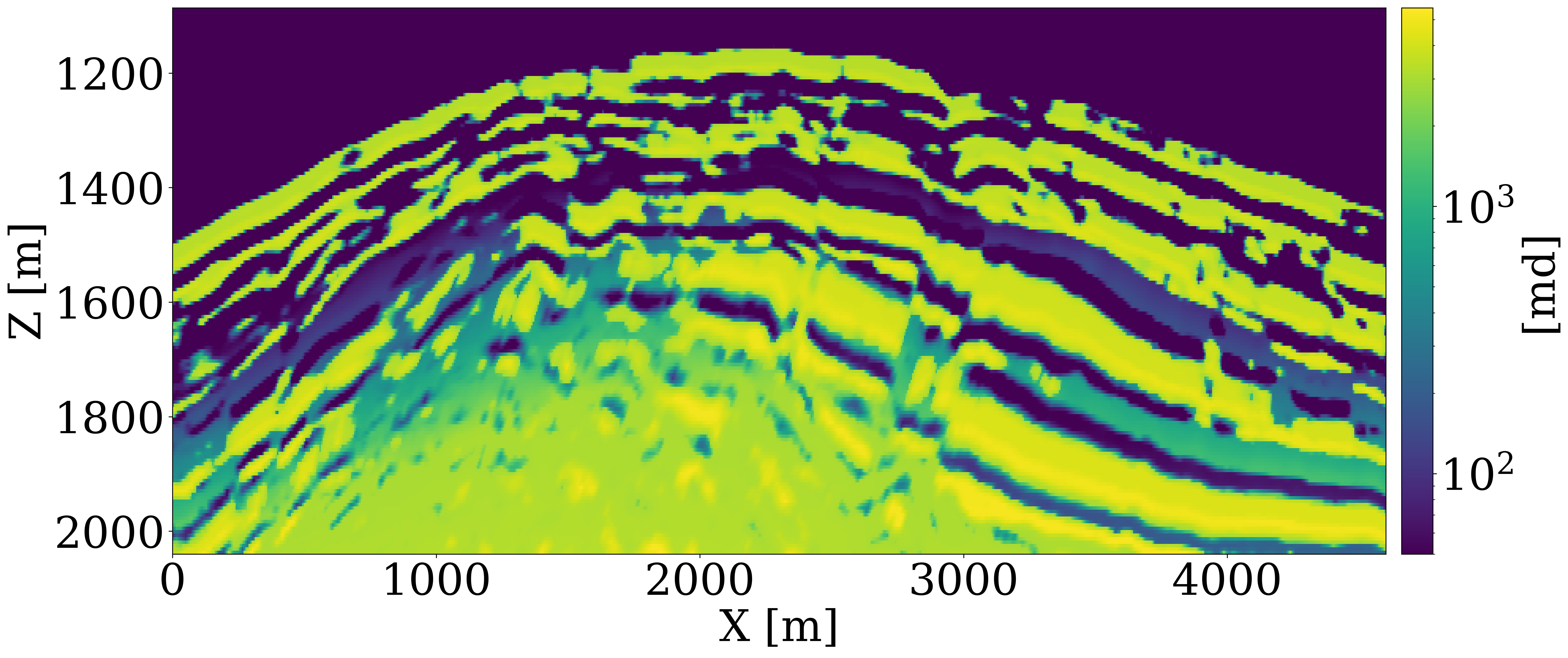
Using five vintages of prestack time-lapse seismic surveys, we aim to invert for the spatial distribution of permeability. To this end, we utilize the aforementioned 2D slice of the velocity model, included in Figure 1 (a), where the orange region signifies the storage unit. Since the Compass model only includes velocities and densities and no permeability or porosity values, we build a fully heterogeneous ground truth permeability model, displayed in Figure 1 (b), by assuming the elementwise relationship in Equation 2, between the entries of the brine-filled velocity model, \(\mathbf{c}_p\), in \(\mathrm{km/s}\), and the horizontal permeability, \(\mathbf{K}\), in millidarcies (md)¹. \[ \mathbf{K} = \begin{cases} 3000 \exp(\mathbf{c}_p-4) \quad \text{if}\quad \mathbf{c}_p\geq 4 \\ 0.01\exp(25.22(\mathbf{c}_p-3.5)) \quad \text{if}\quad \mathbf{c}_p\geq 3.5 \\ 0.01\exp(\mathbf{c}_p-3.5) \quad \text{else} \end{cases} \tag{2}\]

Because the baseline seismic Compass model is derived from well and imaged seismic, it contains subtle changes in the seismic properties related to sub-wavelength interference. The above elementwise relationship between the seismic velocity and permeability ensures that the derived permeability model shares the same spatial heterogeneity as exhibited by the seismic baseline. By construction, it also features significant permeability contrasts within different layers within the storage unit. The low-permeability layers range from approximately \(10^{-3}\) to \(1\) md, while the high-permeability layers vary between \(600\) to \(6000\) md. The histogram of the common logarithm of the permeability model is shown in Figure 1 (c), which demonstrates that the permeability values do not follow log-normal distribution. A CO₂ injection well, marked with a dark blue \(\star\), is placed centrally to inject supercritical CO₂ for 25 years at a constant rate of two million metric tons per year. We assume the porosity and the kv/kh ratio to be constant and given by 25% and 10%, respectively. The simulation of compressible and immiscible two-phase flow, where CO₂ displaces brine in porous rocks, is performed using a fully implicit method implemented in JutulDarcy.jl (Møyner and Bruer 2023; Yin, Bruer, and Louboutin 2023). The boundary of the CO₂ plume at the 25th year is depicted in grey in Figure 1 (a). After converting the CO₂ saturation into seismic velocity models, \(\mathbf{v}\), via the patchy saturation model, acoustic time-lapse seismic data is generated with constant density for five vintages at years 5, 10, 15, 20, and 25 using Devito (Louboutin et al. 2019; Luporini et al. 2020) and JUDI.jl (Witte et al. 2019; Louboutin, Witte, et al. 2023), employing a Ricker wavelet with a central frequency of 20 Hz. The well-bore source and receiver geometries are shown in Figure 1 (a).

3.1 Sensitivity with respect to starting models

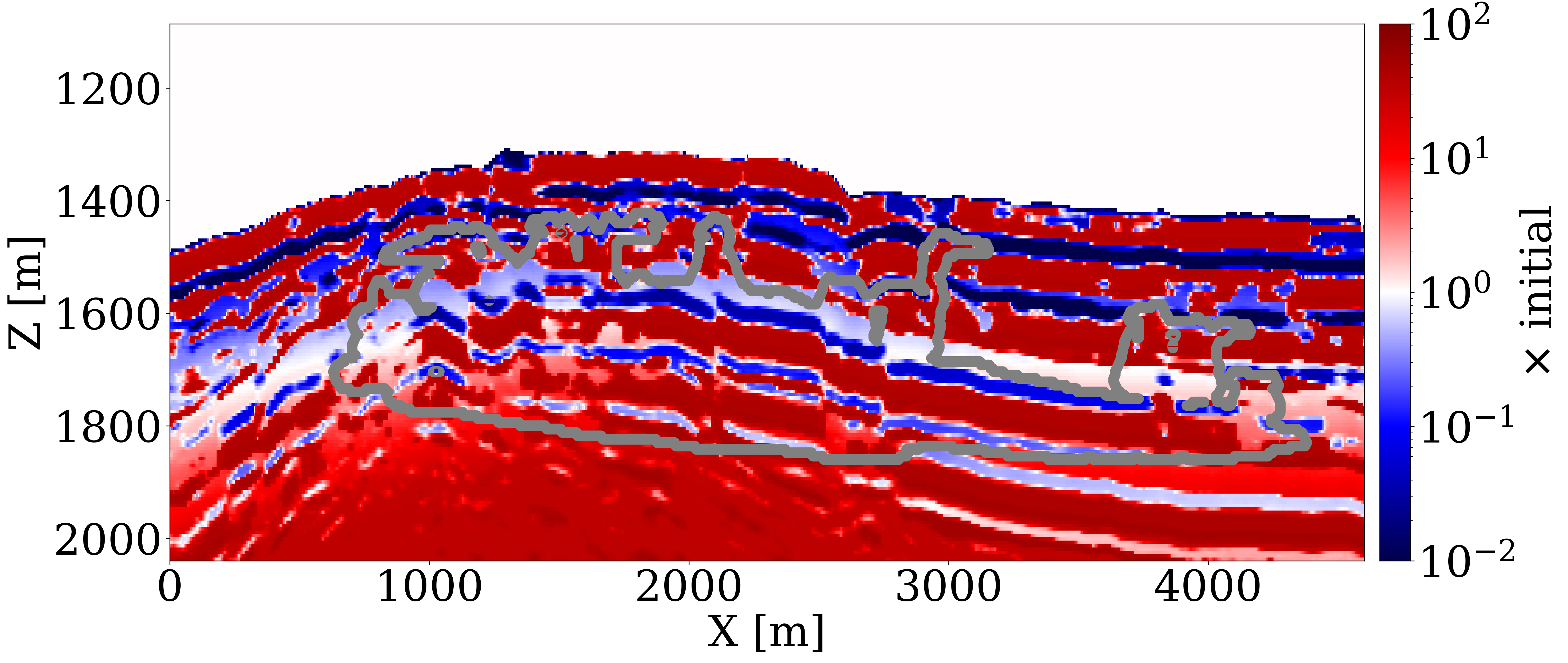
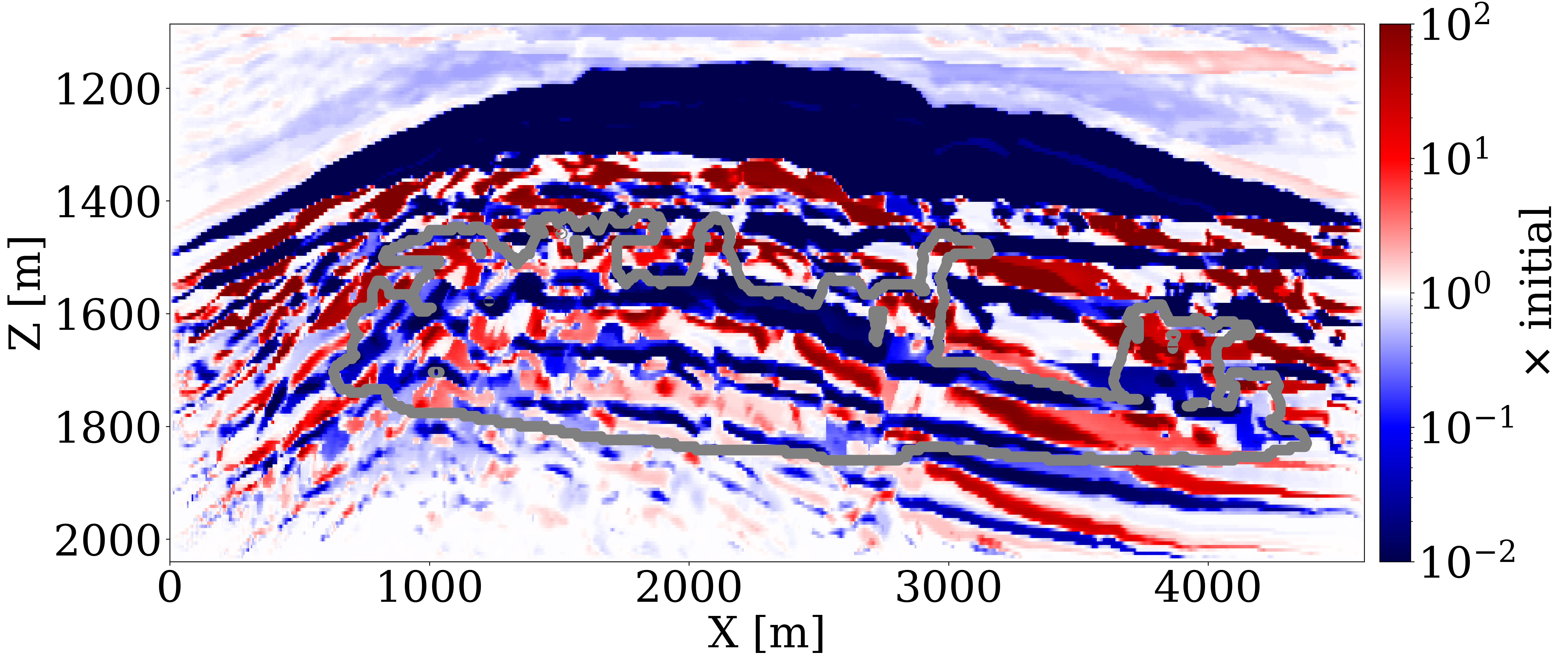
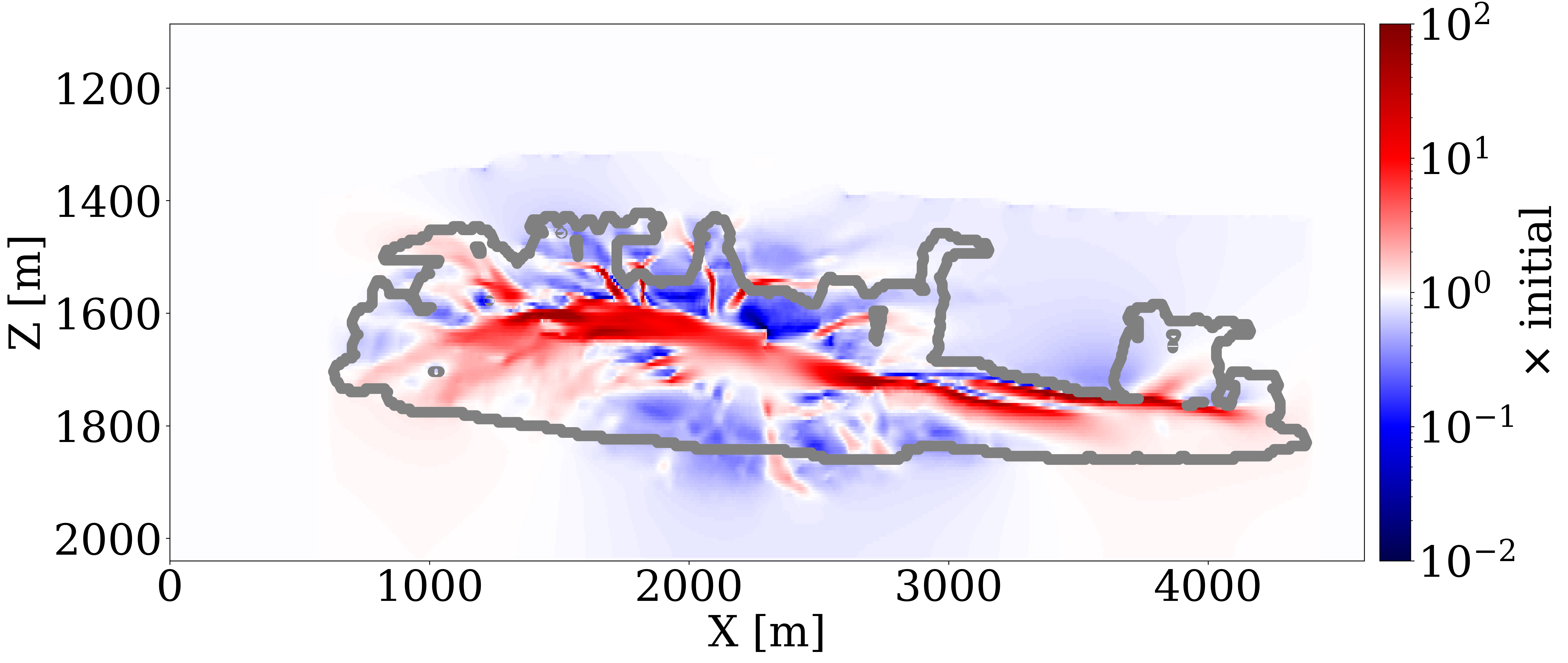
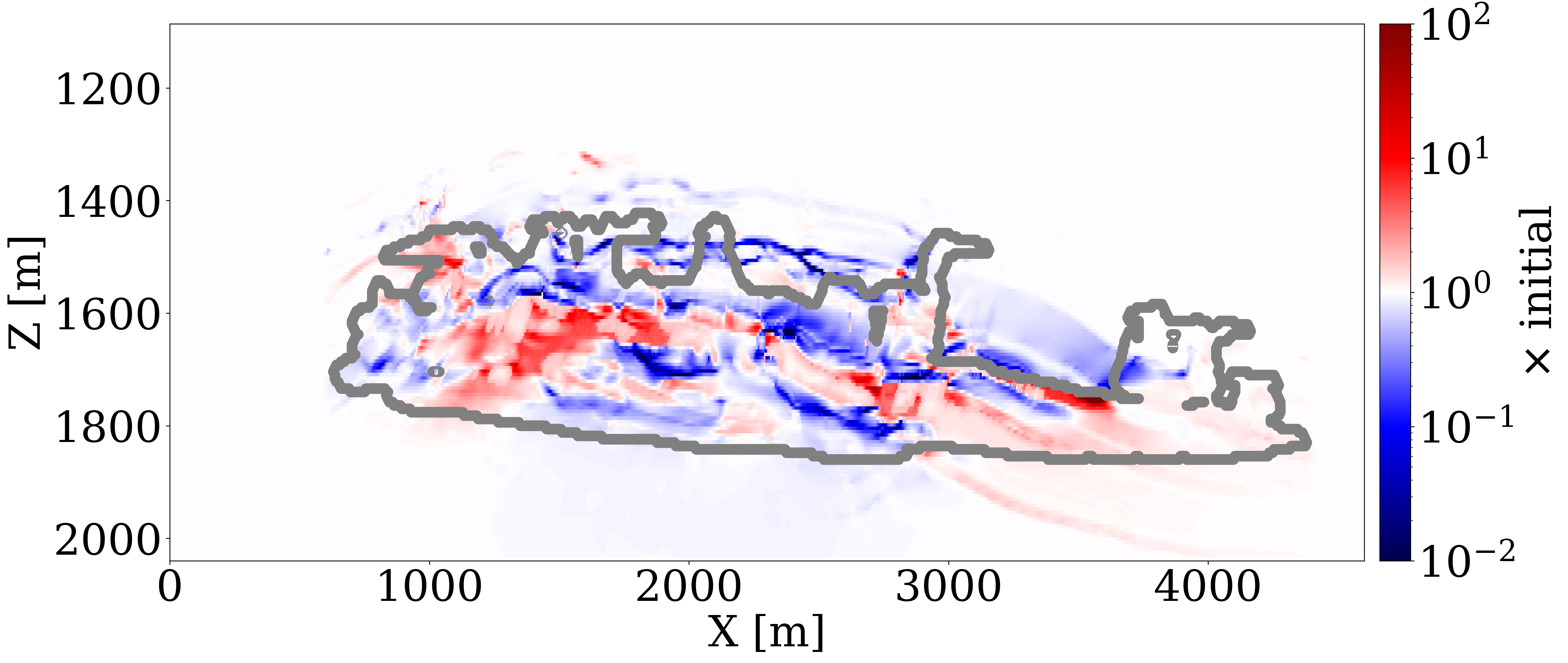
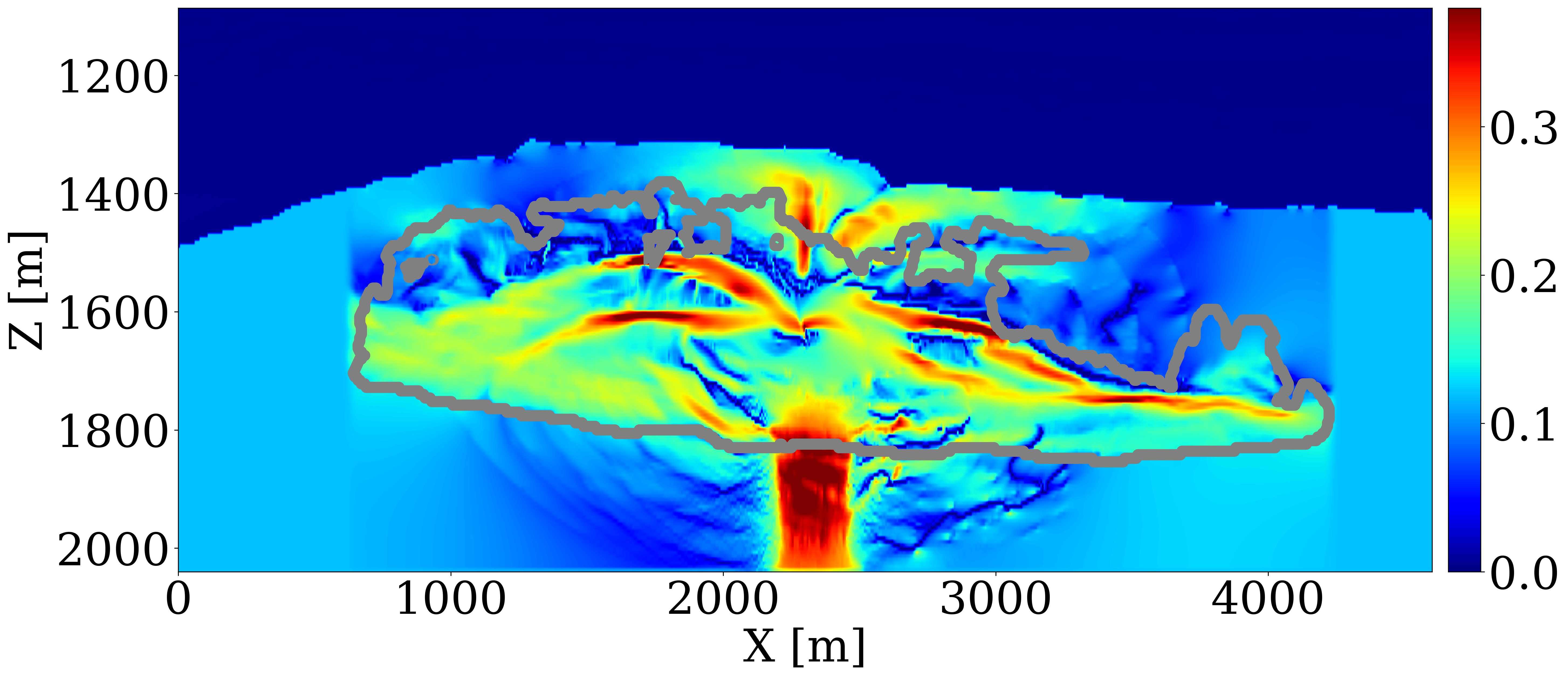
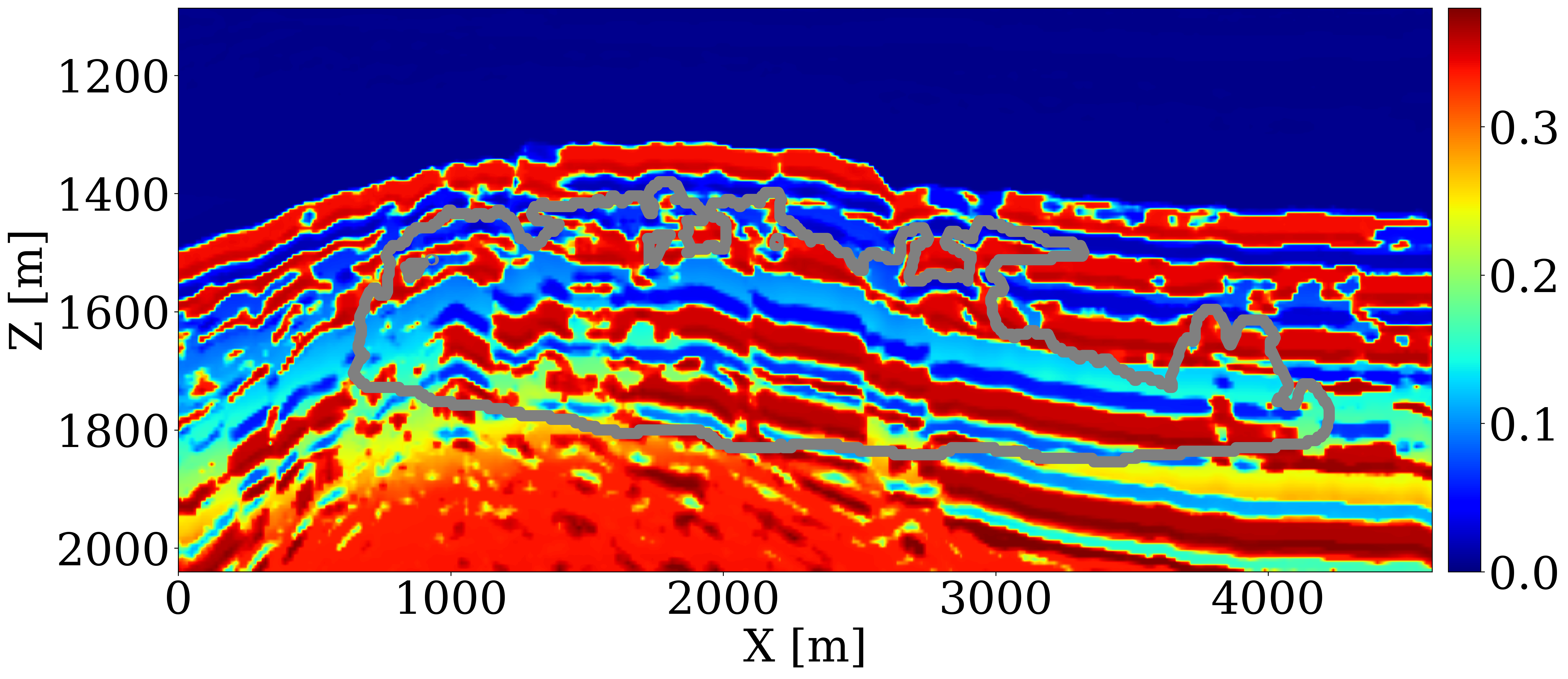
To evaluate the efficacy of our end-to-end inversion framework, particularly its sensitivity to initial permeability models, we examine two distinct initial permeability models. In case 1, the initial permeability model, shown in Figure 3 (a), features homogeneous permeability values (\(100\mathrm{md}\)) across the entire reservoir. This model allows us to explore the extent of permeability updates achievable from a non-informative permeability model. In case 2, we apply a spatial distortion (Bloice, Stocker, and Holzinger 2017) to the unseen ground truth permeability in Figure 1 (b) to obtain the initial permeability model, shown in Figure 3 (b). The values of different permeability layers are near accurate, but the positions are misplaced.

In both cases, we employ a methodological shortcut often referred to as committing an “inversion crime”, where the data generation and inversion processes share the same computational kernel. This ideal setup is used here to show what is ideally achievable by this inversion framework. To add a layer of realism, we incorporate 8 dB of incoherent band-limited Gaussian noise into the observed time-lapse datasets, which severely contaminates the seismic signal in the time-lapse difference.

To invert for the permeability model, we run 100 iterations of stochastic gradient descent (SGD), starting with Figure 3 (a) and Figure 3 (b). During each iteration, we randomly draw four sources out of the total of 32 sources to calculate the misfit and the gradient with respect to permeability model (Herrmann et al. 2013). This amounts to 12.5 datapasses through the entire time-lapse seismic dataset. We display permeability updates in logarithmic scale for both cases, in Figure 3 (e) and Figure 3 (f), respectively. Additionally, Figure 3 (c) and Figure 3 (d) offer a visualization of “ideal” updates by showing the logarithmic differences between the ground truth and the initial permeability models.

The following observations can be made: First, the permeability updates are primarily confined to areas directly influenced by the CO₂ plume’s flow, as delineated by the gray curves. This outcome is expected since the time-lapse variations in wave properties are attributed to changes in fluid saturation exclusively. Consequently, without additional information, this inversion method does not alter permeability values outside the CO₂ plume’s extent where the flow of CO₂ has not occurred. Second, the inverted permeability within the CO₂ plume largely reflects the trend of the ground truth permeability model. In case 1, the framework successfully identifies major permeability layers — both high and low (depicted in red and blue, respectively) at approximately \(1600\,\mathrm{m}\) depth — accurately capturing their depth and lateral distribution in alignment with the actual layers. In case 2, the inversion process introduces high-resolution details to the layers affected by the plume, aligning well with the ideal updates shown in Figure 3 (d). Despite these successes, the full magnitude of permeability contrasts is not entirely captured, pointing to the inherently ill-posed nature of permeability inversion (Zhang, Jafarpour, and Li 2014), necessitating workflows that include uncertainty quantification for future investigations (Gahlot et al. 2023).

(a)

(b)

(c)

(d)

(e)

(f)

Figure 3: Permeability inversion results for cases 1 and 2. (a)(c)(e) display the initial permeability model in case 1, the logarithmic ratio of the ground truth permeability (Figure 1 (b)) to the initial one, and the logarithmic ratio of the inverted permeability to the initial one. (b)(d)(f) display the same but for case 2 with a distorted initial permeability model. Gray curve indicates the boundary of the CO₂ plume at the 25th year. “\(\times\) initial” on the caption of the colorbar represents the factor by which the initial permeability is updated.

3.2 Sensitivity with respect to forward modeling errors

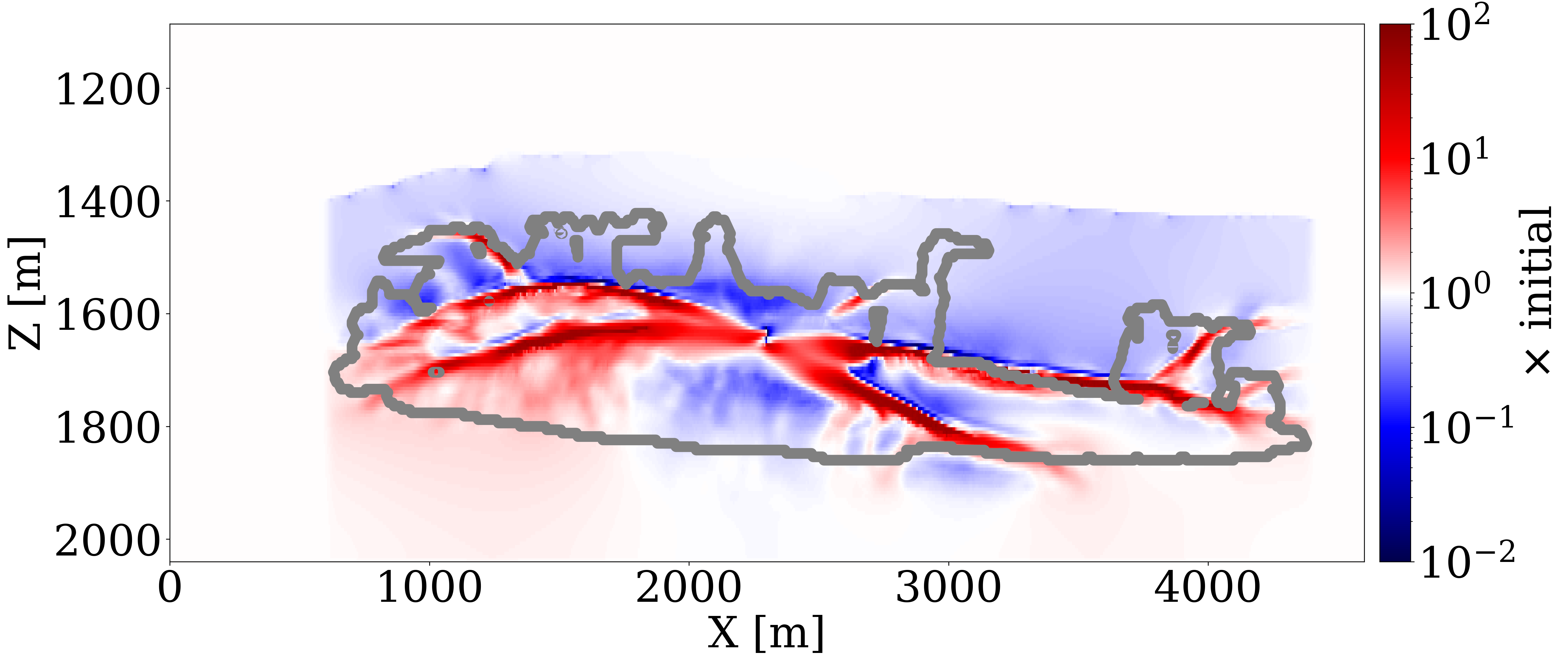
To extend our investigation beyond overly idealized scenarios, we examine the framework’s robustness next, during scenarios that avoid “committing the inversion crime”. A critical area of focus in time-lapse seismic is the error in the brine-filled baseline velocity model before CO₂ injection. Errors in this baseline model, which feeds into the rock physics model, can produce inaccurate velocity models of the CO₂-filled reservoir, leading to inaccuracies in the simulated time-lapse seismic datasets.

To construct an inaccurate but realistic baseline velocity model, we use a Ricker wavelet with central frequency of \(20\,\mathrm{Hz}\) to generate cross-well and surface seismic data before CO₂ injection, and employ the SGD method to run 10 datapass of FWI with a kinematically correct but smooth initial velocity model to obtain the inverted velocity model depicted in Figure 4 (a). This imperfect brine-filled velocity model is subsequently fed into the rock physics model, \(\mathcal{R}\), for permeability inversion (case 3).

We employ the initial permeability model from Figure 3 (a) to assess the impact of modeling errors on the inversion results. The update to the permeability, shown in logarithmic scale in Figure 4 (b), reveals some artifacts outside the CO₂ plume area due to the modeling inaccuracies. Additionally, a high permeability zone within the plume is slightly misplaced when compared to the updates in Figure 3 (e), yet the overall trend of permeability changes is correctly captured.

Following this permeability update, we proceed with reservoir simulations using the updated permeability models to assess the corrections made to the CO₂ plume predictions. This step is crucial for validating the practical utility of the inversion framework for real-world seismic monitoring scenarios.

(a)

(b)

Figure 4: Permeability inversion results for case 3. (a) Inverted brine-filled baseline velocity used in permeability inversion. (b) The logarithmic ratio of the inverted permeability to the initial one. Gray curve indicates the boundary of the CO₂ plume at the 25th year.

3.3 CO₂ plume estimation and forecast

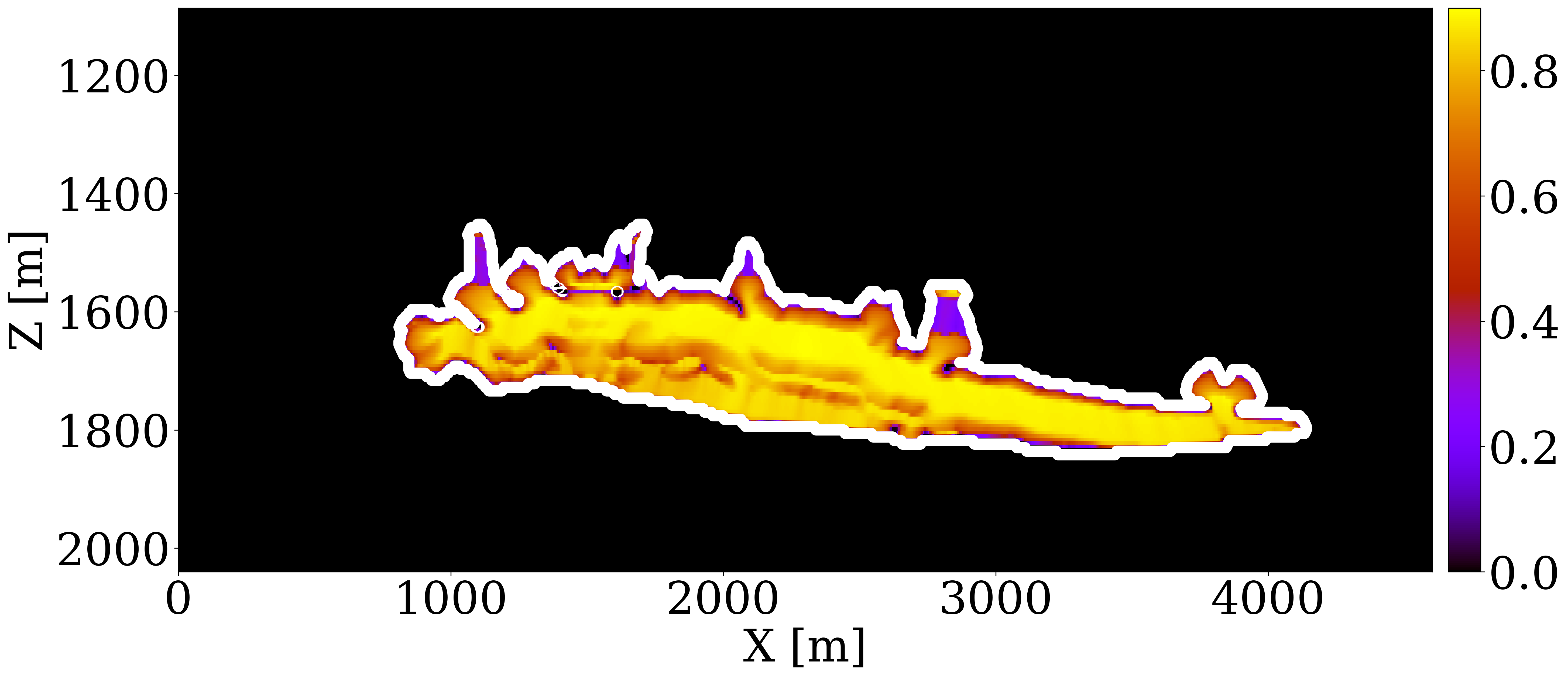
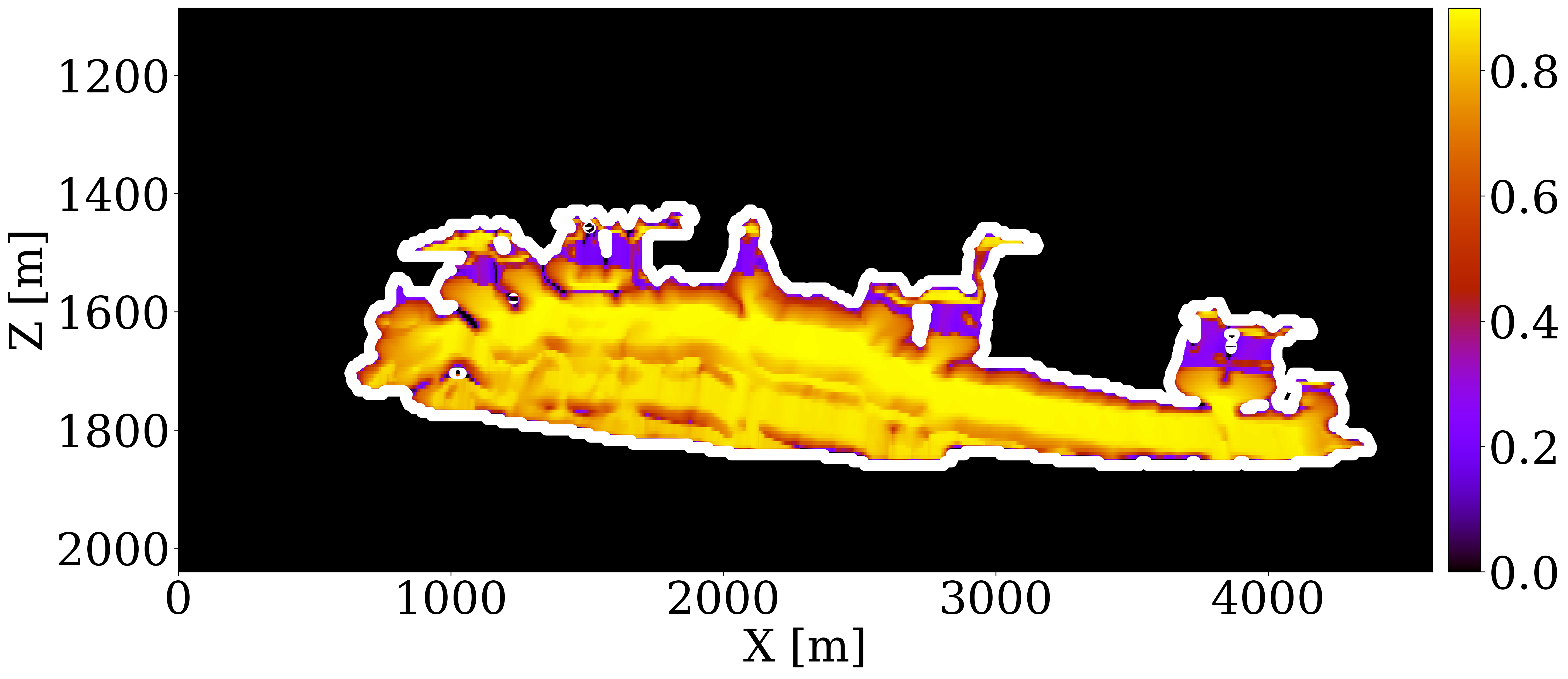
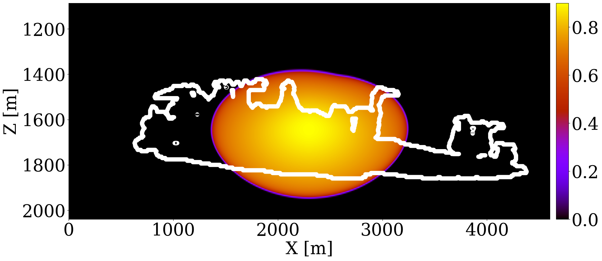
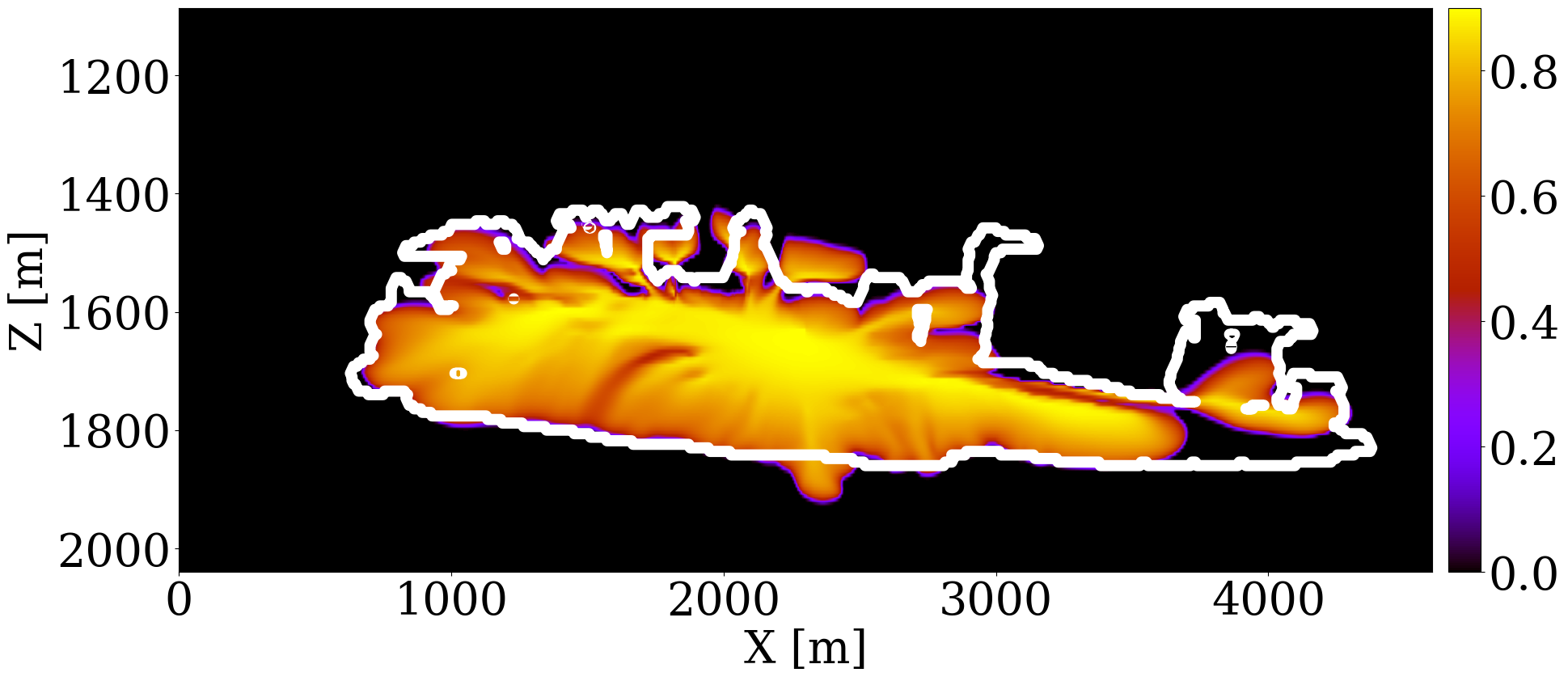
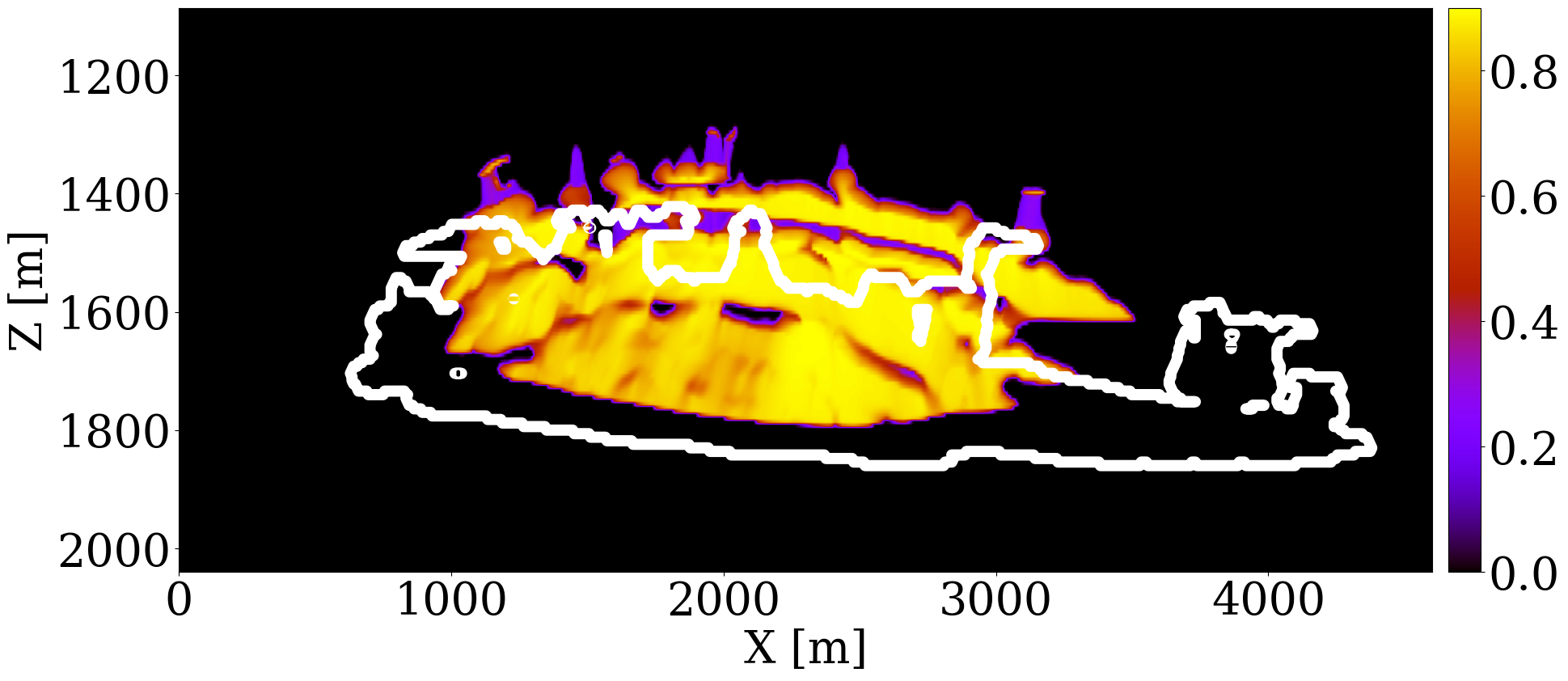
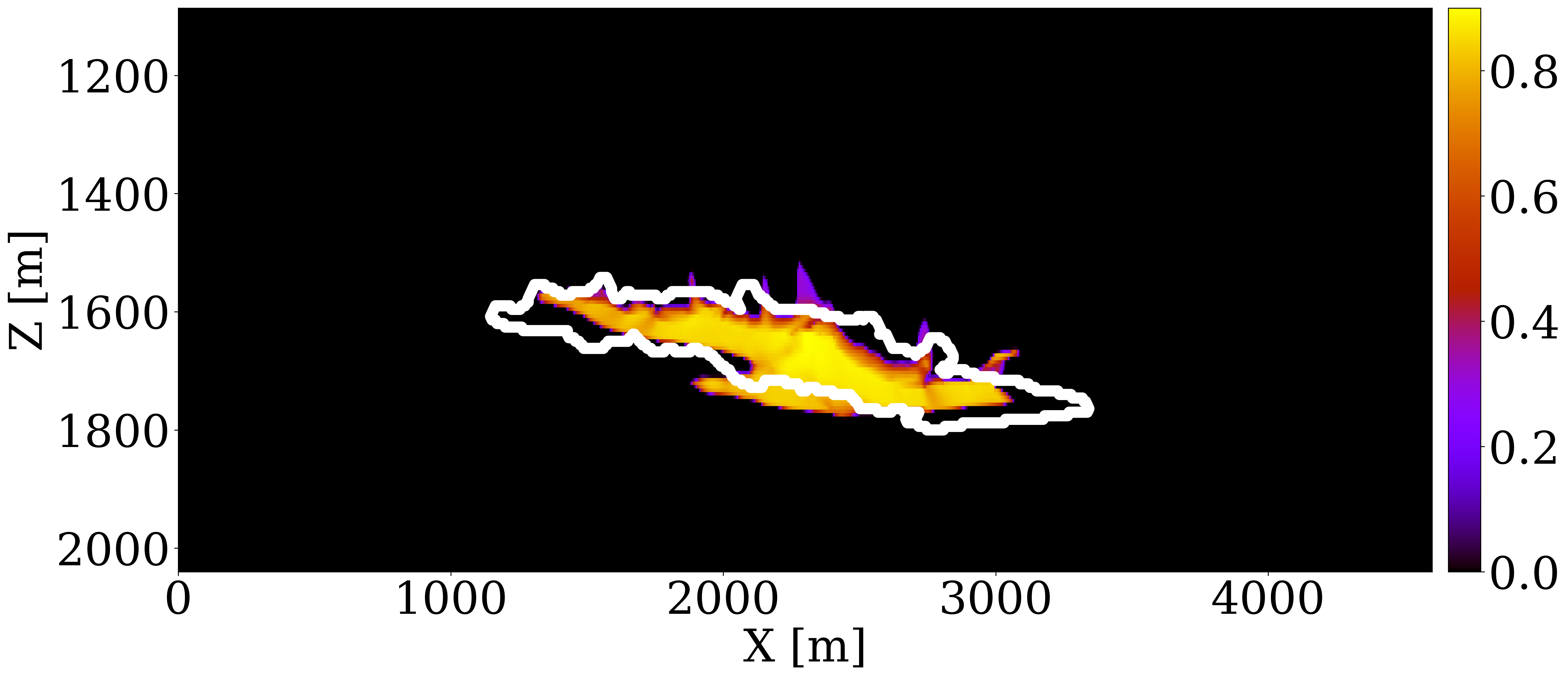
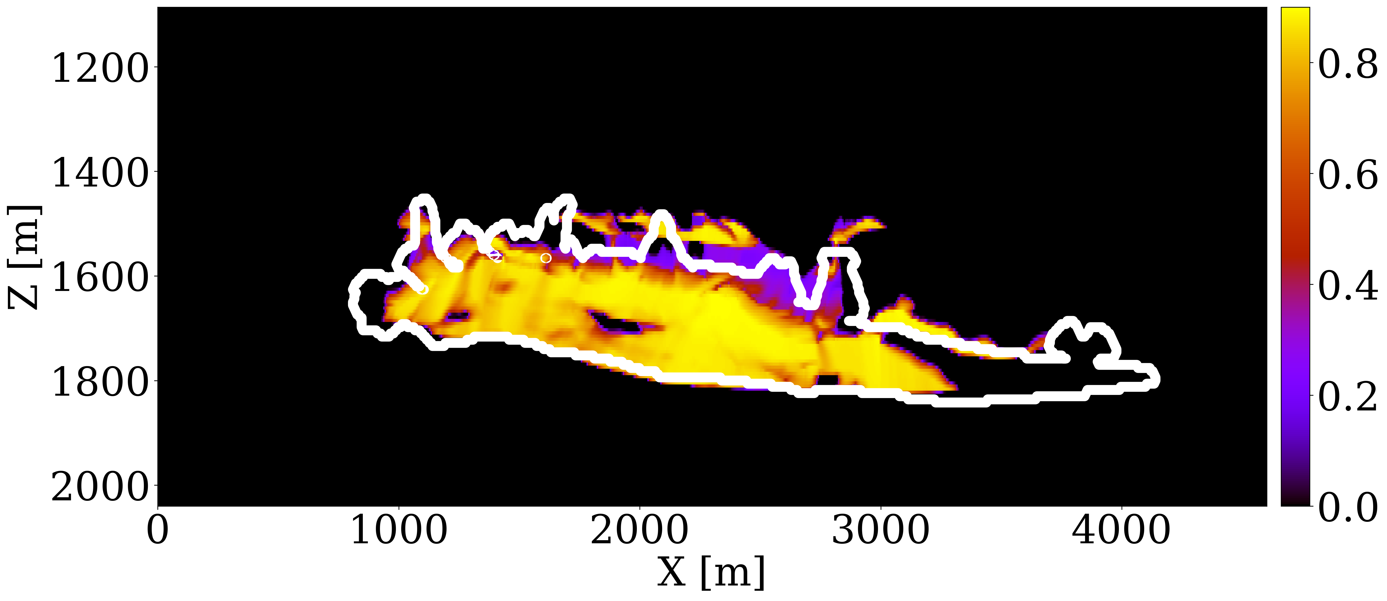
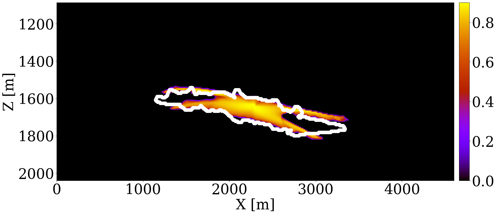
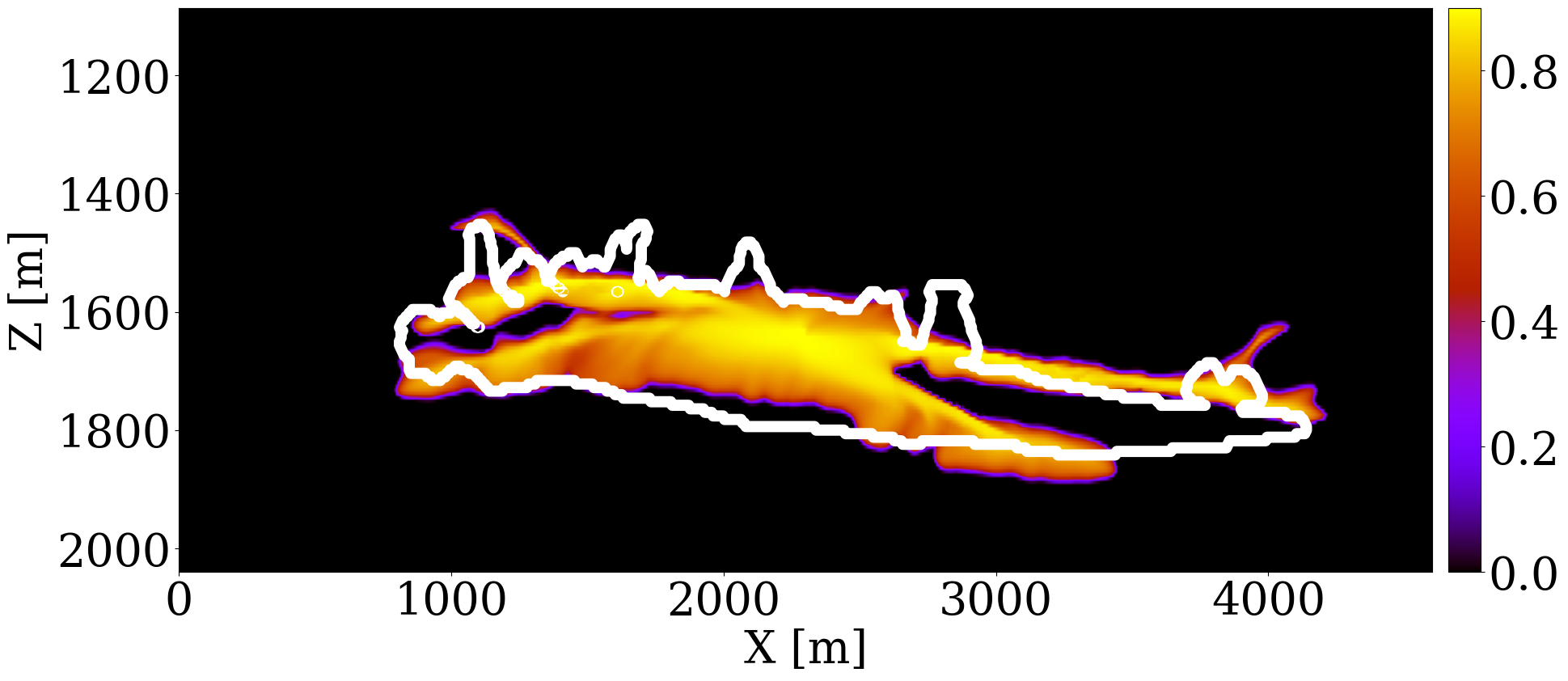
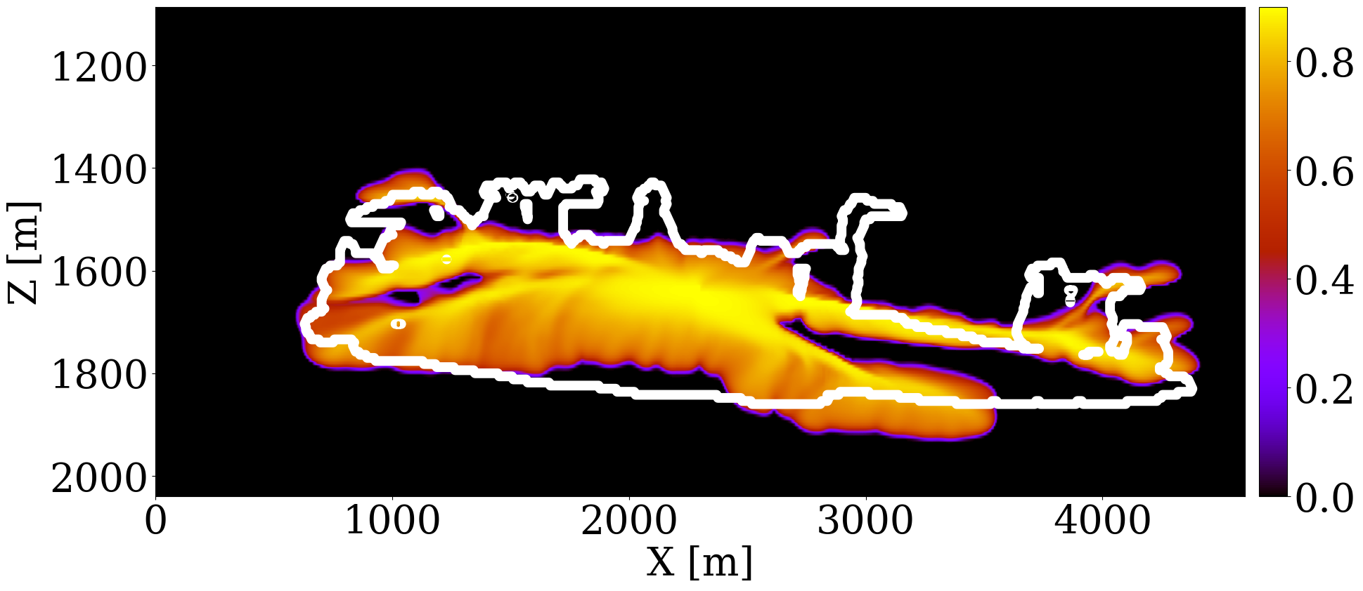
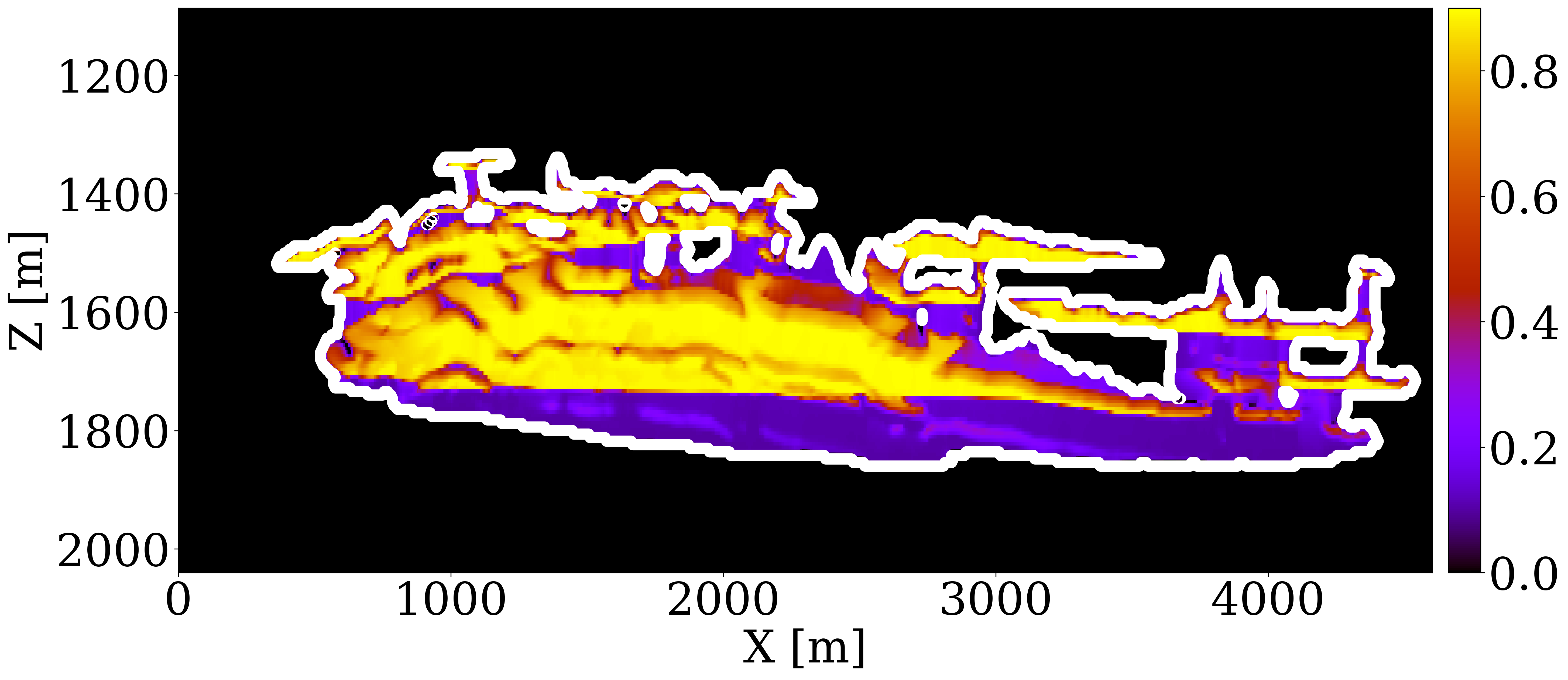
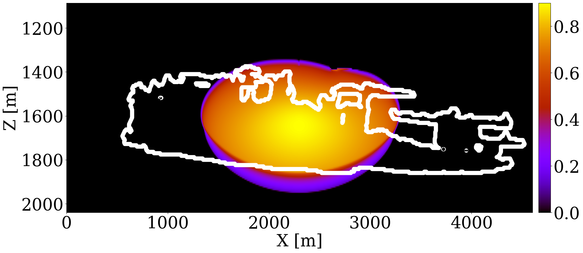
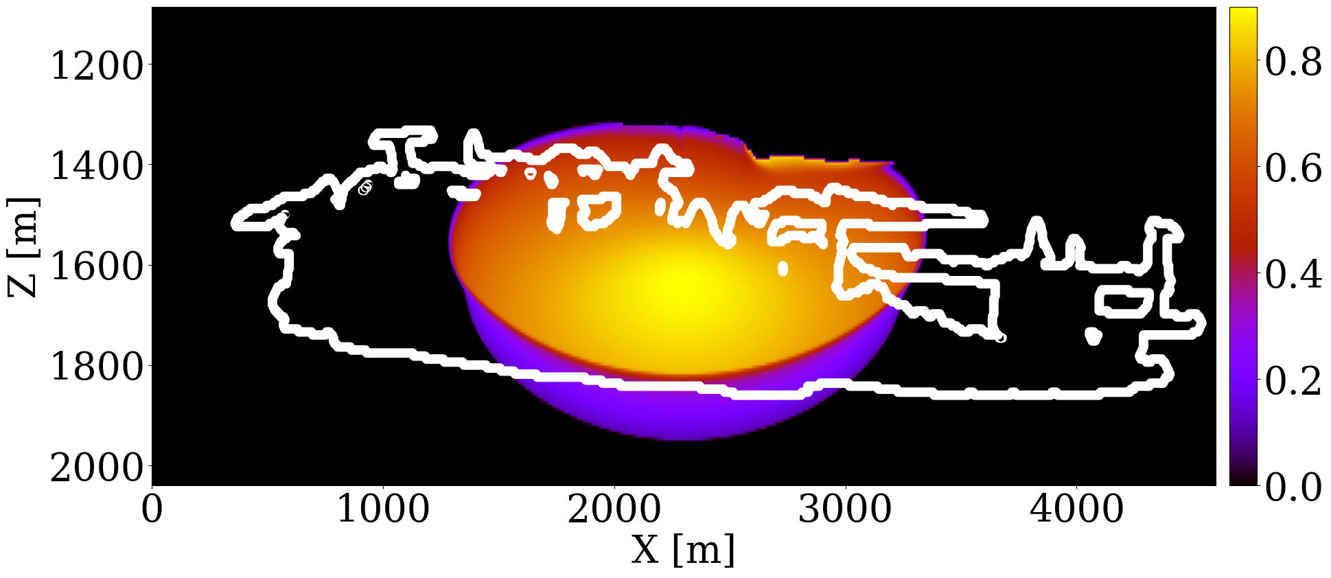
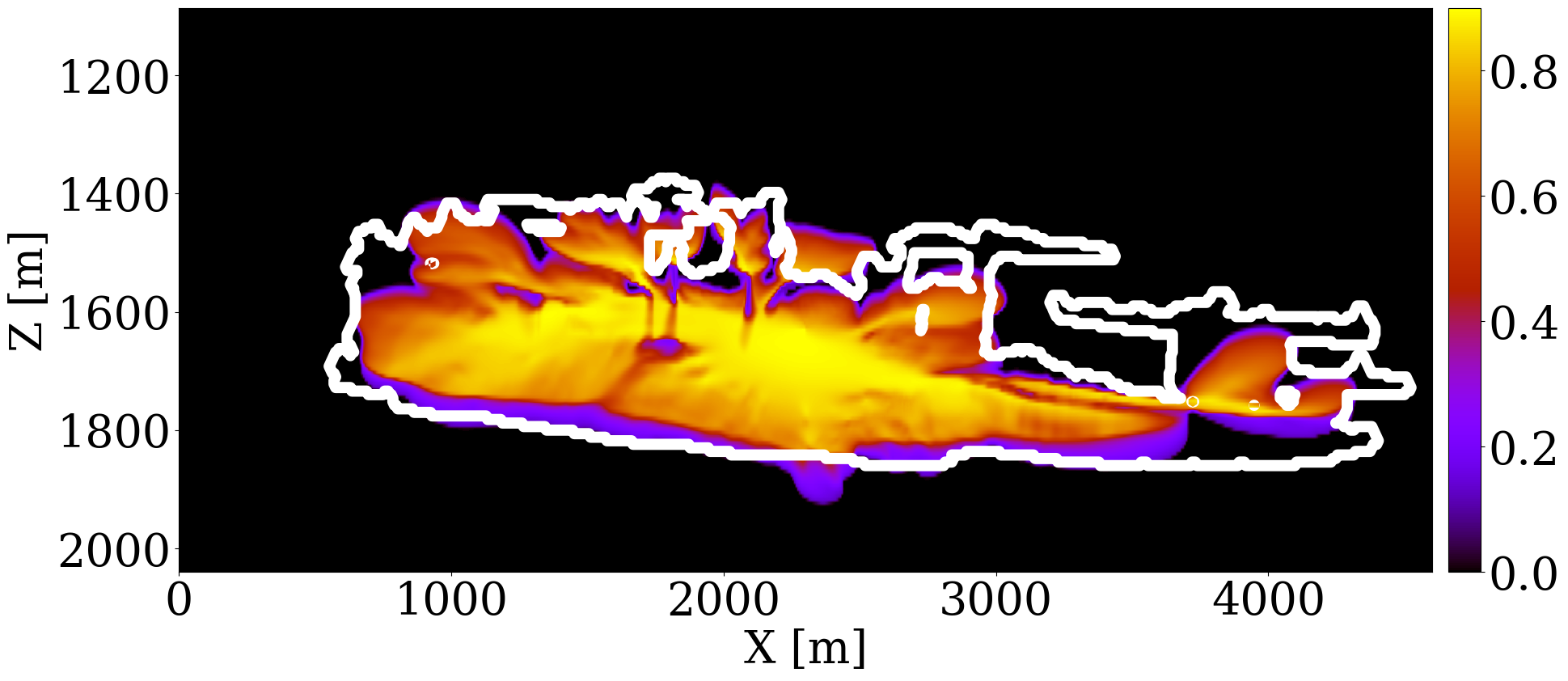
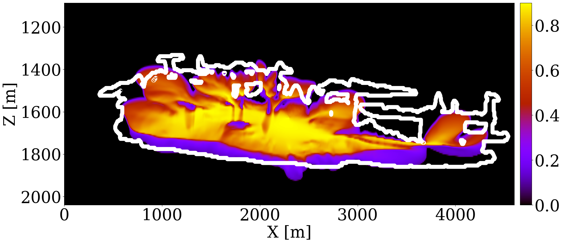
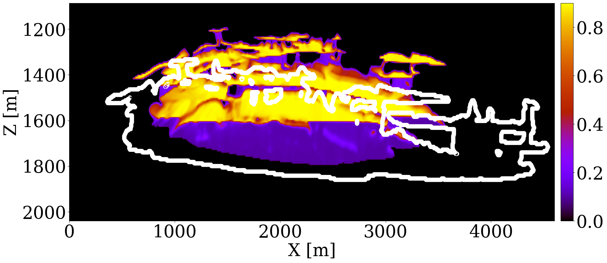
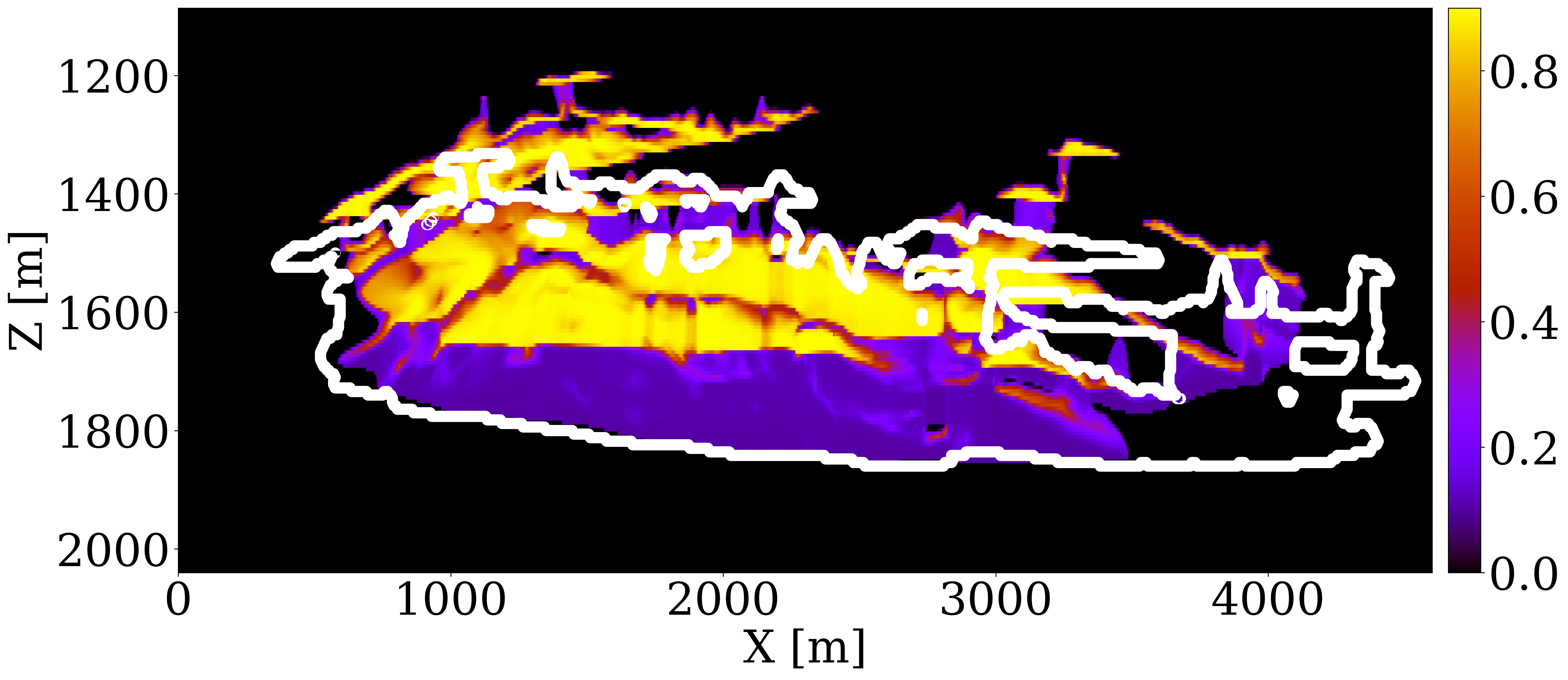
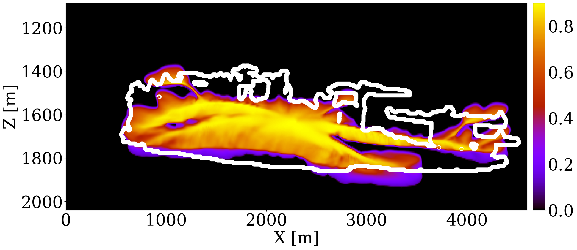
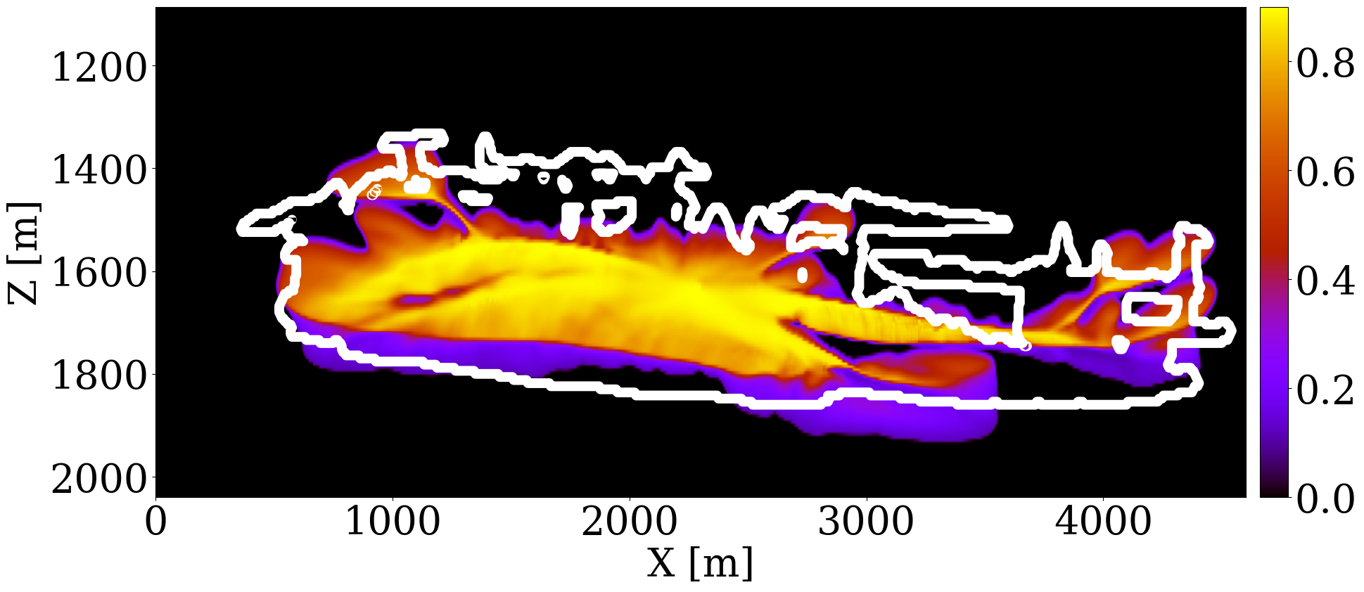
The primary objective of our end-to-end inversion framework is to accurately estimate reservoir permeability, a crucial step towards the ultimate goal of predicting CO₂ saturation both historically and in the near future. Based on initial, inverted, and ground truth permeability models, we conduct a quality control involving CO₂ saturation simulations, as depicted in Figure 5. Across all simulations, we note substantial improvements in predictions of the CO₂ plume shape, closely aligning with the boundaries of the ground truth CO₂ plume. Notably, the initial simulations significantly misjudged the lateral spread of the CO₂ plume. The corrections applied through the updated permeability models, however, yield accurate representations of the plume’s lateral extent.

Figure 5: Predicted CO₂ saturation for 5th, 15th, and 25th years, shown in first, second, and third columns, respectively. The first row shows the (unseen) ground truth CO₂ saturation. The second and fourth rows show the saturation predicted with initial permeability models in Figure 3 (a) and Figure 3 (b), respectively. The third, fifth, and sixth rows show the updated saturation after updating the initial permeability models by Figure 3 (e), Figure 3 (f), and Figure 4 (b), respectively. The boundaries of the (unseen) ground truth CO₂ saturation are shown in white curves.

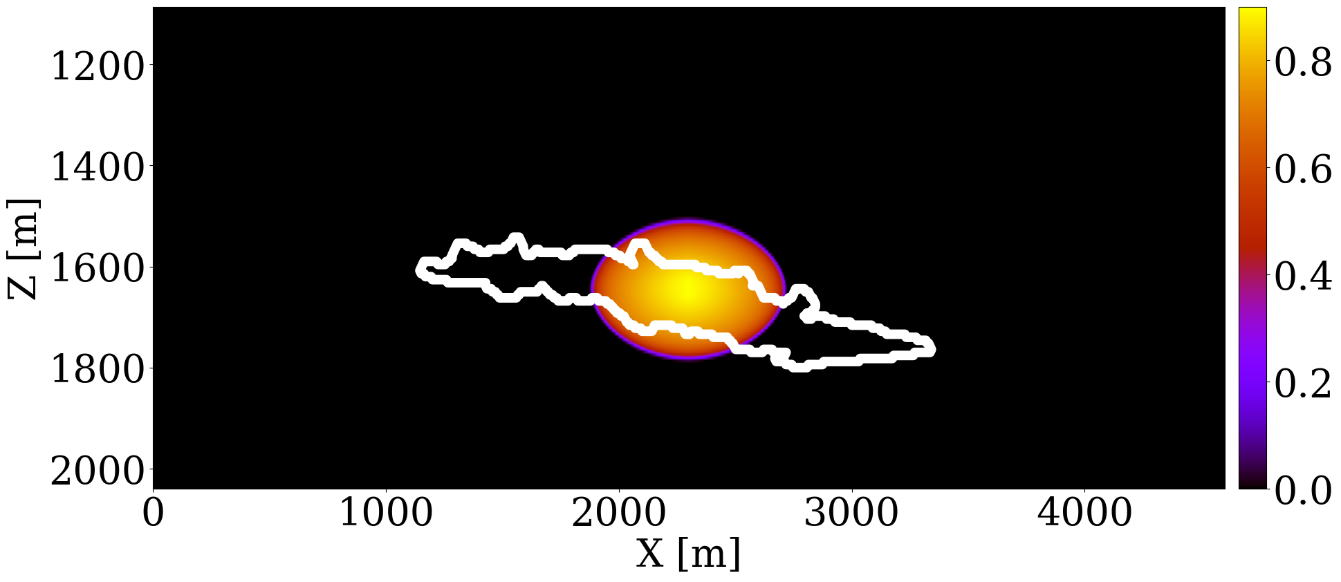
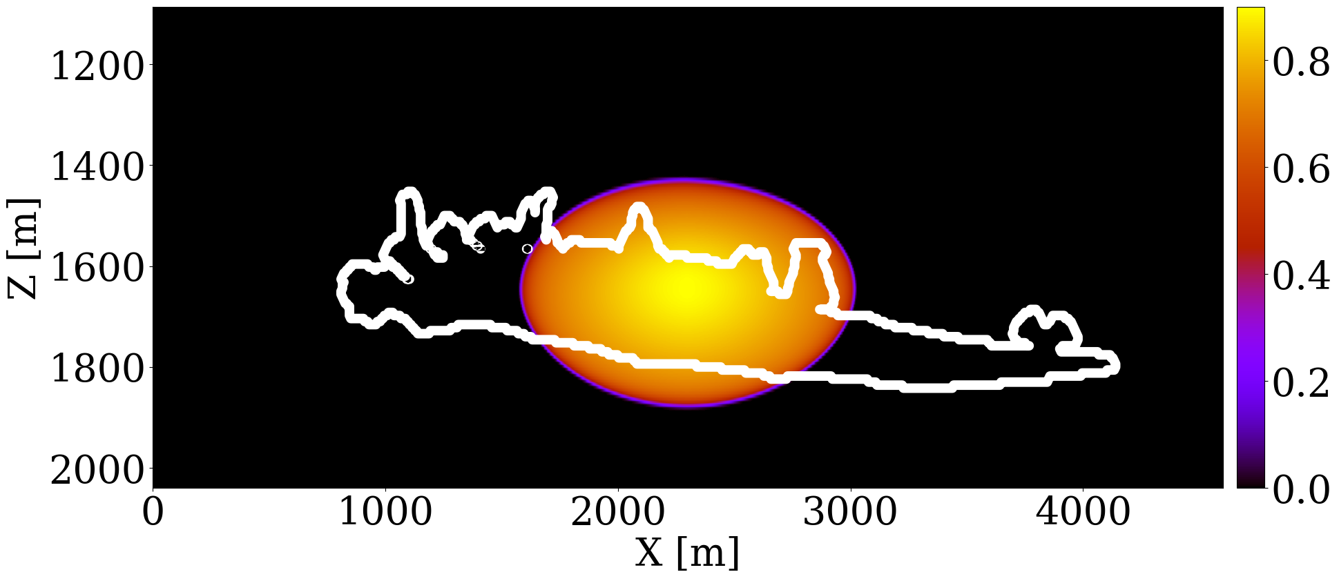
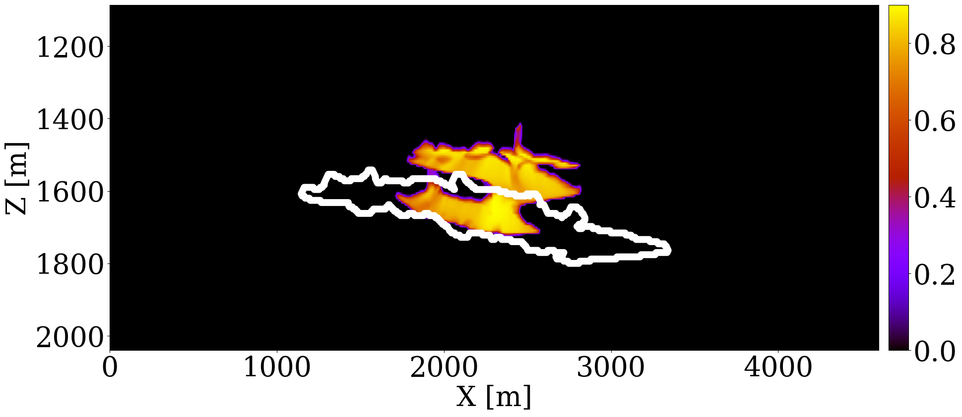
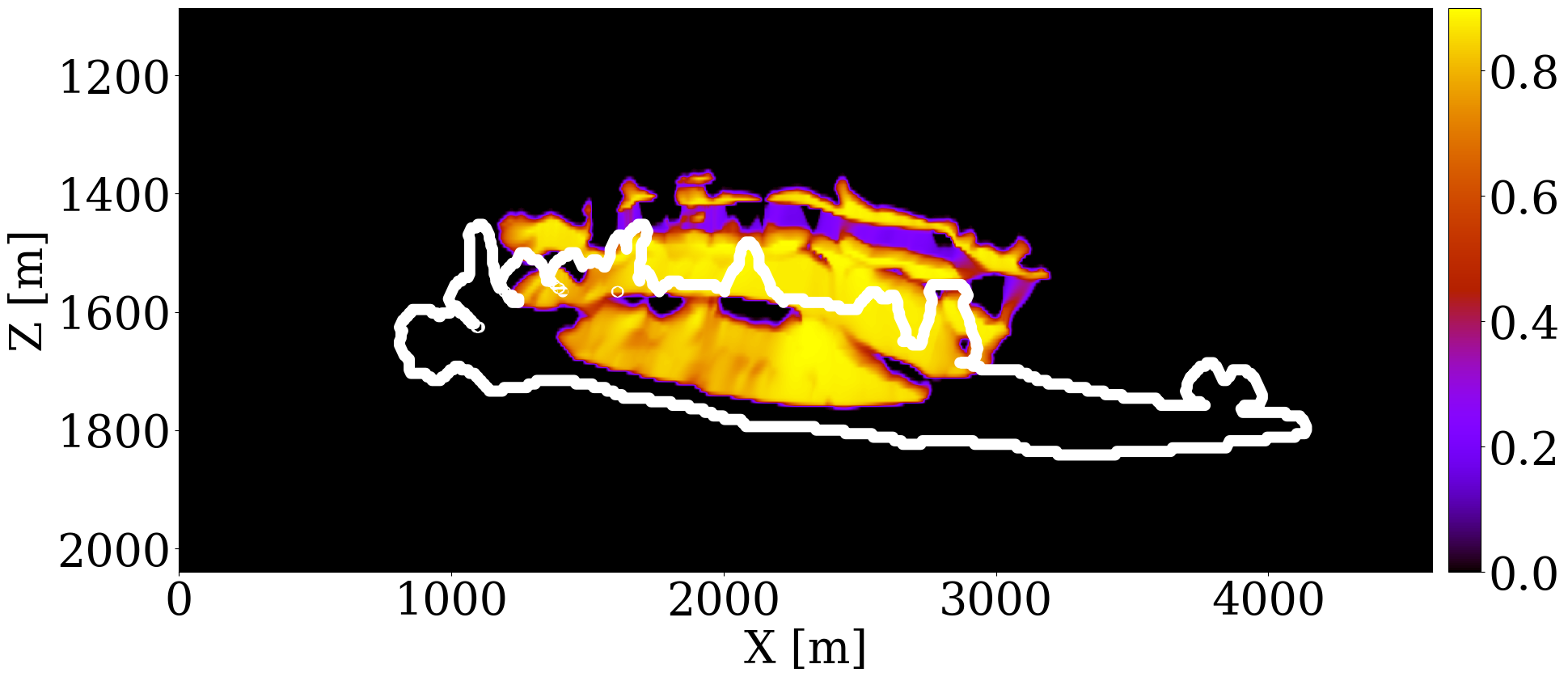
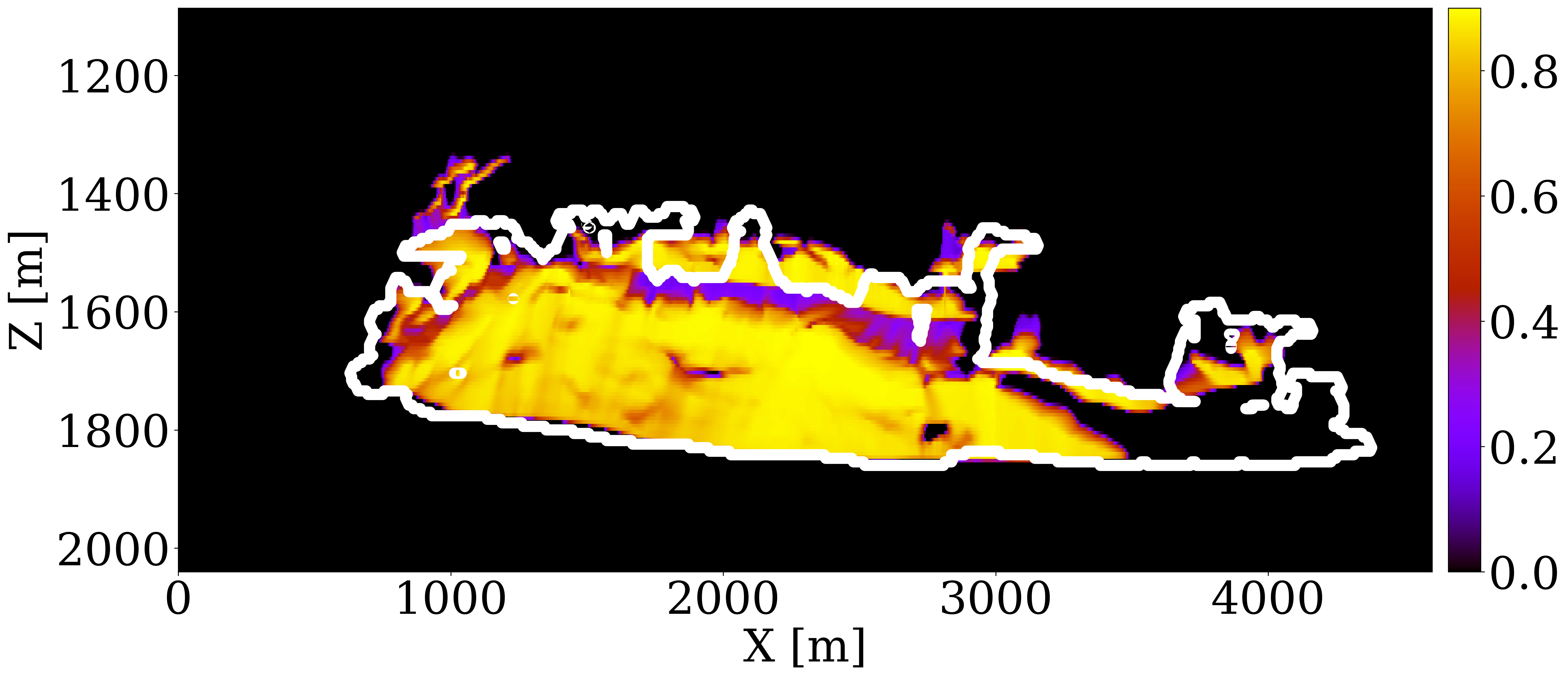
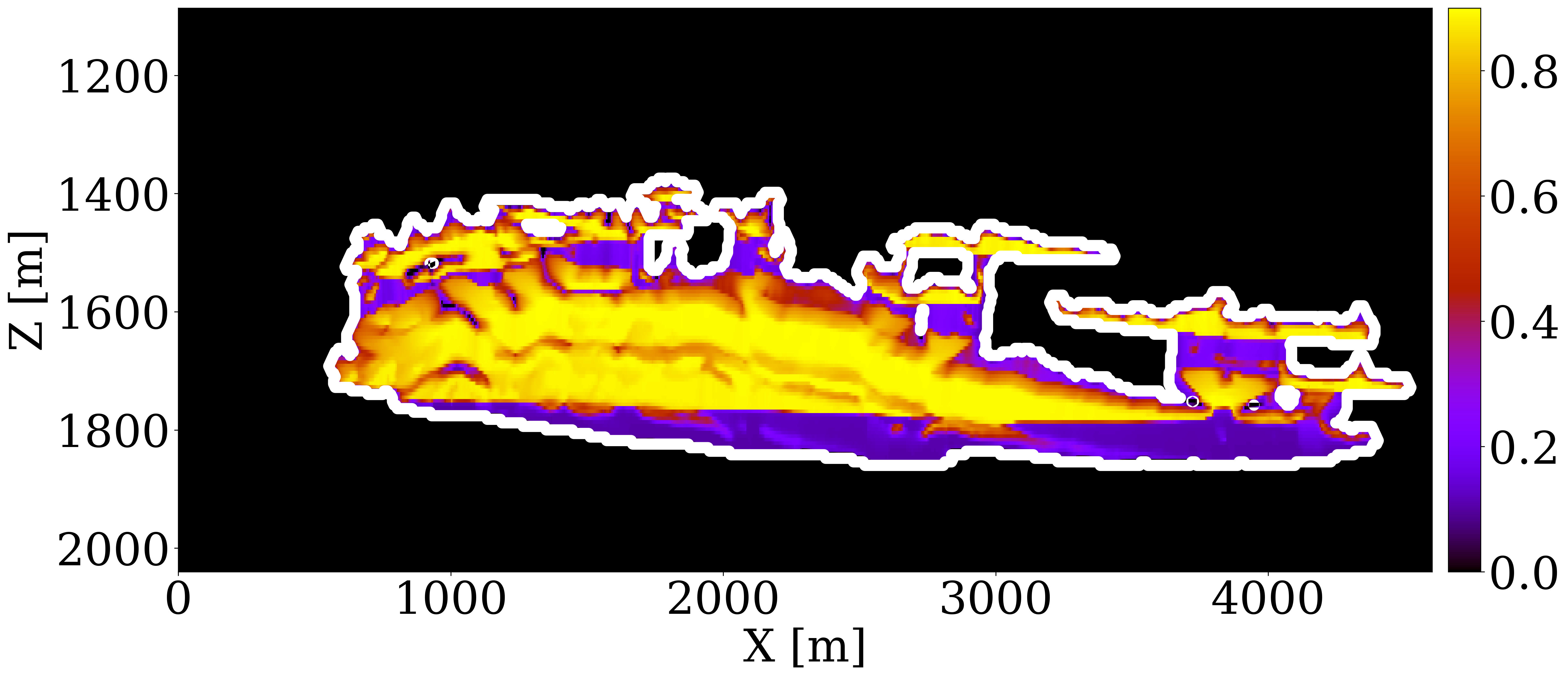
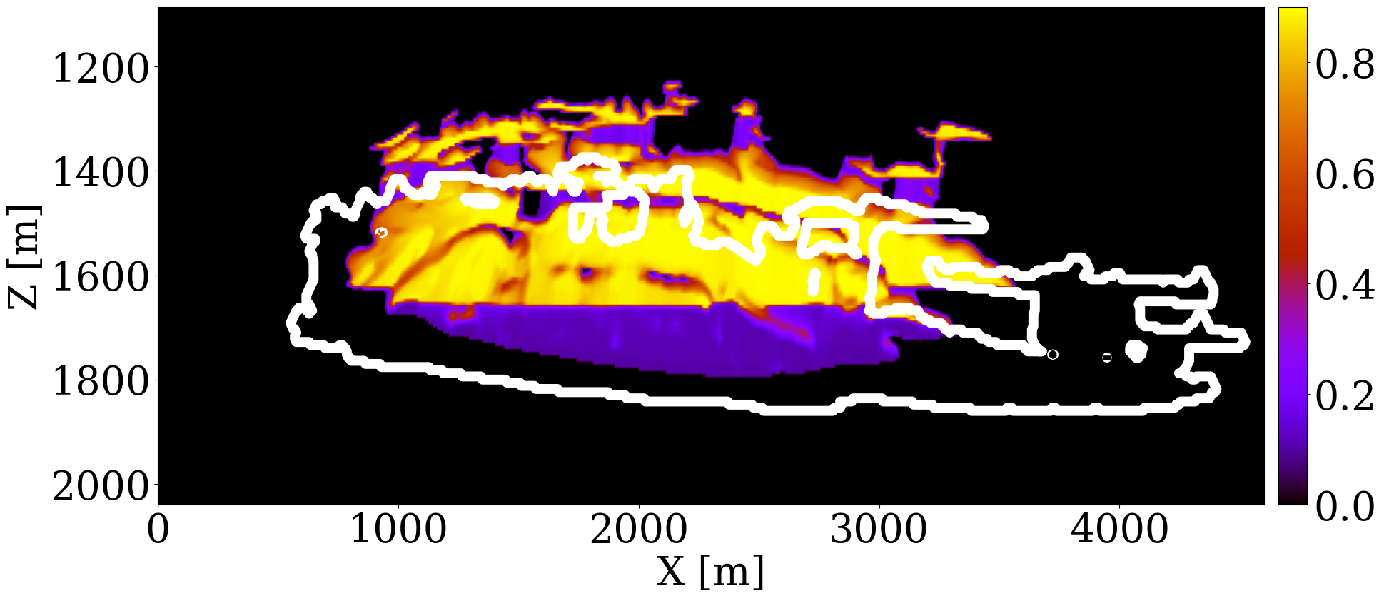
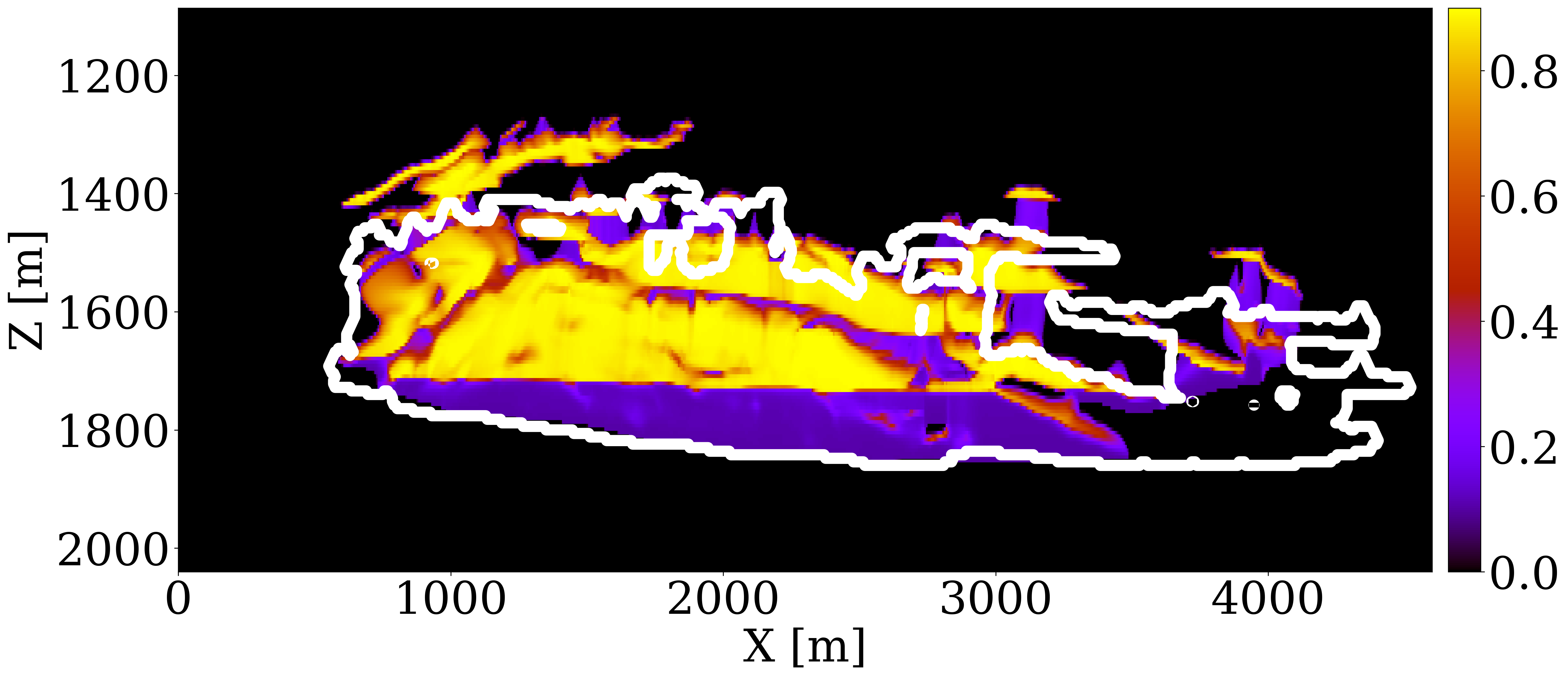
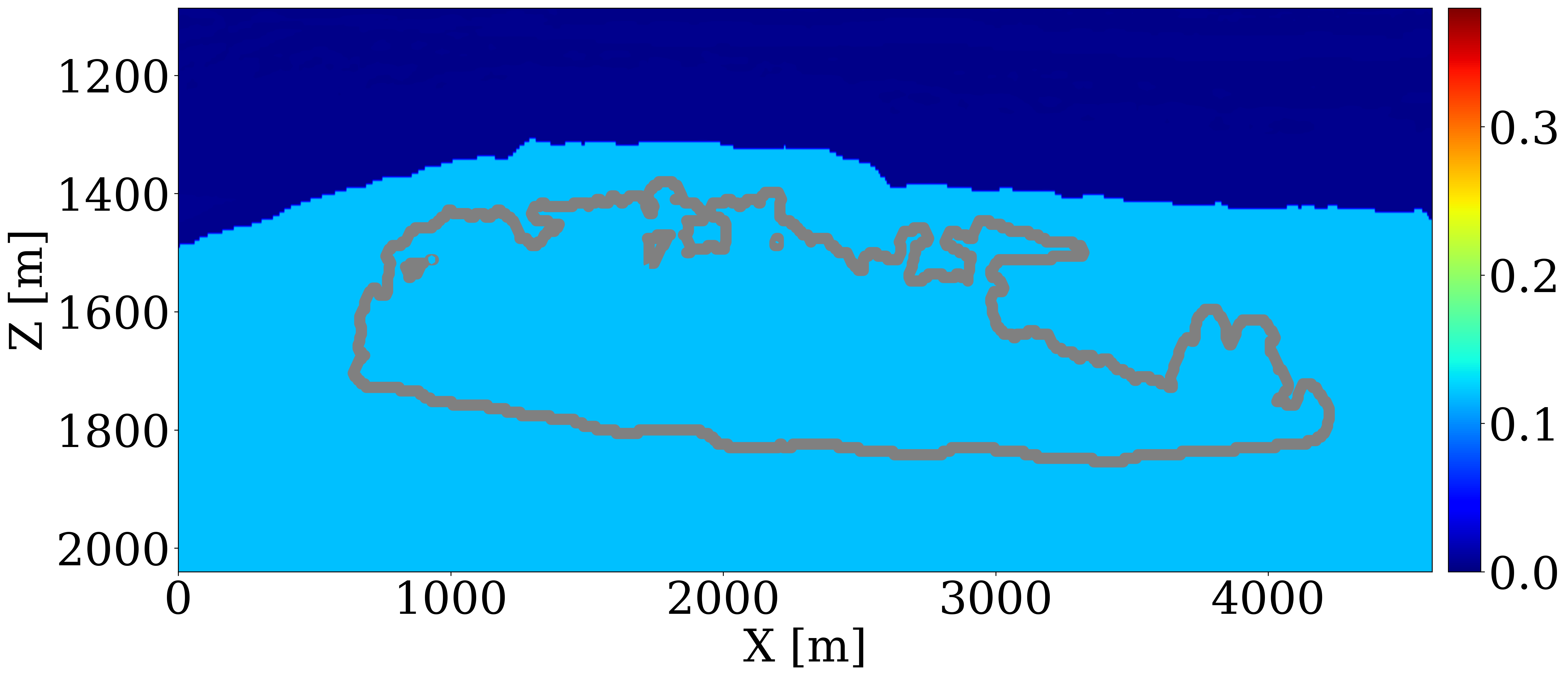
Expanding our analysis to future forecasting, Figure 6 illustrates the predicted movement of the CO₂ plume over a 40-year period, following a 25-year injection phase, without further CO₂ injection or seismic observations. During this forecasted period, the CO₂ plume primarily ascends due to buoyancy, while a portion (approximately 10%) remains trapped in the pore spaces, indicated in purple. This phenomenon, known as residual trapping (Rahman et al. 2016), is a critical factor in assessing the long-term storage capabilities of GCS projects. Initial forecasts tend to underestimate the extent of CO₂ sequestration through residual trapping. In contrast, simulations driven by the updated permeability models not only provide a more accurate estimation of the permanently stored CO₂ volume but also closely match the ground truth CO₂ plume’s boundaries, even without collecting further monitoring data.

Figure 6: CO₂ plume forecasts for 45th and 65th years, shown in first and second columns, respectively. The ordering of the rows remains the same as Figure 5. Purple regions display the CO₂ plume permanently stored via the residual trapping mechanism.

3.4 Multiparameter inversion

While case 1-3 demonstrate the performance of the inversion framework for permeability estimation, further scrutiny is in order to investigate its performance when multiple parameters are unknown and need to be jointly estimated. To this end, we design case 4 where spatial distributions of both porosity and permeability are unknown. While permeability only appears in the two-phase flow equations, porosity appears as an input not only in the two-phase flow reservoir simulator, \(\mathcal{S}\), but also in the patchy saturation model, \(\mathcal{R}\). This results in a more challenging inverse problem because porosity affects more than one physics-based forward models in Figure 2, and because there can be crosstalk in the gradient calculations during the inversion.

As a proof of concept, we simplify this multiparameter inversion problem by assuming that the porosity, \(\boldsymbol{\phi}\), and the horizontal permeability, \(\mathbf{K}\), are related by the following elementwise Kozeny-Carman relationship (Costa 2006):

\[ \mathbf{K} = \mathcal{T}(\boldsymbol{\phi})=3.65 \times 10^4 \frac{\boldsymbol{\phi}^3}{(1-\boldsymbol{\phi})^2}. \tag{3}\]

Following this relationship, we artificially create a ground truth porosity model, shown in Figure 7 (c), according to the permeability values in Figure 1 (b), and then use the ground truth permeability and porosity models to simulate CO₂ saturation, velocity models, and the five time-lapse seismic datasets. During inversion, we parameterize permeability by porosity according to Equation 3, and minimize the following objective function to invert for the porosity:

\[ \underset{\boldsymbol{\phi}}{\operatorname{minimize}} \quad \|\mathcal{F}\left(\mathcal{R}\left(\boldsymbol{\phi}, \mathcal{S}\left(\boldsymbol{\phi}, \mathcal{T}\left(\boldsymbol{\phi}\right)\right)\right)\right)-\mathbf{d}\|_2^2. \tag{4}\]

The scalable and differentiable programming framework, proposed by Louboutin, Yin, et al. (2023), allows for effortless and accurate gradient calculation with respect to porosity, \(\boldsymbol{\phi}\), which otherwise requires labor-intensive and error-prone derivation of cross-gradient terms by hand. We initialize the reservoir with homogeneous porosity values of \(12\%\), shown in Figure 7 (a). After 100 iterations of SGD, the inverted porosity is shown in Figure 7 (b). While some layers in the inverted porosity are slightly misplaced in this preliminary study, the overall trend of porosity is adequately estimated in the center of the model.

(a)

(b)

(c)

Figure 7: Porosity inversion in case 4. (a) Initial porosity. (b) Inverted porosity. (c) Unseen ground truth porosity. The gray curve delineates the shape of the CO₂ plume at the 25th year.

4 Limitations

While our case studies offer promising insights, it is crucial to acknowledge the assumptions underpinning our approach and recognize the inherent limitations that merit further investigation. Additionally, we explore the potential for integrating this 4D processing workflow with other reservoir characterization and management strategies.

4.1 Reservoir simulation

Our study assumes known values for all multiphase flow model parameters, including relative permeability functions, residual water saturation, temperature and capillary pressure. These parameters were kept constant in the simulations to isolate the impact of permeability on seismic data, but there can be significant rock-dependent variations in practice. A multiparameter inversion, indicated by the preliminary case study in case 4, is worthwhile for future investigation to extend this inversion framework through joint estimation of these parameters. Further exploration is also required to understand the crosstalk between these parameters. In addition, our assumption that supercritical CO₂ miscibility in the resident brine is low could be removed by considering a compositional flow model that introduces additional uncertain parameters. The feasibility of such approaches hinges on the availability of a differentiable reservoir simulator, like JutulDarcy.jl, or the use of deep neural networks to approximate the physics of multiphase flow (Grady et al. 2023; Louboutin, Yin, et al. 2023; Yin, Orozco, et al. 2023) and serve as a surrogate during inversion. Moreover, multiphase flow equations may not hold in scenarios involving CO₂ leakage, necessitating robust leakage detection methodologies (Erdinc et al. 2022; Yin, Erdinc, et al. 2023).

4.2 Rock physics

The case studies currently ignore the pressure effect on the wave properties (MacBeth 2004; MacBeth, Floricich, and Soldo 2006). While this can be justified for some GCS projects where the pressure change is relatively subtle, the inversion framework can be extended to honor the relationship between pressure and wave properties, and include geomechanical effects (Chen et al. 2020; Nagao et al. 2023). The patchy saturation model may also not fully capture the complexities of real-world reservoirs (Allo and Vernik 2024), indicating a need for calibration of the rock physics model against actual reservoir and seismic data.

4.3 Wave physics

The omission of updates to the brine-filled baseline velocity model represents a simplification that warrants further exploration. Future research could extend the framework to jointly update this baseline alongside permeability, incorporating additional parameters like shear velocity and density, which are currently ignored in the modeling and inversion. Quantifying uncertainties in velocity (Yin et al. 2024; Yin, Orozco, and Herrmann 2024; Orozco et al. 2024) and permeability models remains a critical challenge for enhancing the reliability of inversion results.

5 Discussion and conclusion

Our feasibility studies demonstrate the performance of this inversion framework in estimating permeability models directly from multiple prestack time-lapse seismic datasets in a cross-well setting. The recovered horizontal details in the permeability, especially shown in Figure 3 (f) using a \(6\,\mathrm{m}\) grid spacing, highlight the capability of this end-to-end inversion framework to provide high-resolution spatial information of the permeability model. This framework also has the potential to significantly reduce cycle time in 4D processing workflows by avoiding labor-intensive, step-by-step inversion schemes where seismic velocity and CO₂ saturation are subsequently inverted from right to left in Figure 2. Furthermore, the proposed framework differs from conventional workflows (Hatab and MacBeth 2021a, 2021b) by coupling fluid-flow, rock, and wave physics, leveraging the sensitivities of the reservoir simulator through a differential programming software framework (Louboutin, Yin, et al. 2023). By utilizing the rock physics model that links changes in CO₂ saturation to changes in seismic properties, we gain access to these sensitivities from the time-lapse seismic data, allowing us to invert for the permeability directly.

Opportunities for future research remain. This inversion framework can be further enhanced to incorporate multimodal observations, such as a combination of well measurements and seismic data. This enhancement can be readily achieved by integrating additional misfit terms into the objective function, as detailed by Yin, Orozco, et al. (2023). Moreover, the resolution of permeability inversion deserves more exploration. Currently, the inversion is limited to the resolution achievable by seismic methods. Adopting a multimodal data assimilation approach necessitates further studies into the upscaling of the permeability model (Wu, Efendiev, and Hou 2002), which we leave for future work. Additionally, the permeability inversion framework is well-suited for integration with the digital twin framework, as reported by Herrmann (2023) and in other ongoing projects at our research group. When time-lapse seismic and well measurements are collected from the field, performing permeability inversion facilitates more accurate estimations of reservoir properties. These estimations can then be used to forecast the CO₂ plume’s behavior and optimize well injectivity in GCS projects, thereby maximizing injection volumes while minimizing fracturing risks (Gahlot et al. 2024).

6 Data availability

Software with this research can be accessed at http://github.com/slimgroup/TL-FWPI.jl/, with the DOI link https://doi.org/10.5281/zenodo.10910283. The full 3D Compass model is open access with CC BY license, available at ftp://slim.gatech.edu/data/synth/Compass/.

7 Acknowledgements

The authors would like to thank Zhishuai Zhang and the other anonymous reviewer for the thorough reviews and valuable suggestions to our original manuscript. This research was carried out with the support of Georgia Research Alliance, partners of the ML4Seismic Center, and the US National Science Foundation grant OAC 2203821.

The North Sea CO₂ storage project information is taken from the Strategic UK CCS Storage Appraisal Project, funded by the UK Department of Energy and Climate Change, commissioned by the Energy Technologies Institute (ETI), and delivered by Pale Blue Dot Energy, Axis Well Technology, and Costain. The information contains copyright information licensed under ETI Open License.

During the preparation of this work, the authors used ChatGPT to refine sentence structures and improve the readability of the manuscript. After using this service, the authors reviewed and edited the content as needed and take full responsibility for the content of the publication.

Figure 1 (a): Figure 1 (b): Figure 1 (c): Figure 2: Multiphysics forward model. The reservoir simulator, \(\mathcal{S}\), produces \(n_k\) snapshots of time-varying CO₂ saturation, compiled in \(\mathbf{c}\), from the permeability model, \(\mathbf{K}\). The rock physics model, \(\mathcal{R}\), based on the porosity and the brine-filled velocity model, converts each CO₂ saturation snapshot, \(\mathbf{c}_k\), to the altered velocity model, \(\mathbf{v}_k\) . The shaded area highlights the CO₂-induced changes in velocity. Finally, the wave modeling, \(\mathcal{F}\), generates a time-lapse seismic dataset, \(\mathbf{d}_k\), for each velocity model, \(\mathbf{v}_k\). These datasets are collected in the vector, \(\mathbf{d}\). Figure 3 (a): Figure 3 (b): Figure 3 (c): Figure 3 (d): Figure 3 (e): Figure 3 (f): Figure 4 (a): Figure 4 (b): Figure 5: Predicted CO₂ saturation for 5th, 15th, and 25th years, shown in first, second, and third columns, respectively. The first row shows the (unseen) ground truth CO₂ saturation. The second and fourth rows show the saturation predicted with initial permeability models in Figure 3 (a) and Figure 3 (b), respectively. The third, fifth, and sixth rows show the updated saturation after updating the initial permeability models by Figure 3 (e), Figure 3 (f), and Figure 4 (b), respectively. The boundaries of the (unseen) ground truth CO₂ saturation are shown in white curves. Figure 5: Predicted CO₂ saturation for 5th, 15th, and 25th years, shown in first, second, and third columns, respectively. The first row shows the (unseen) ground truth CO₂ saturation. The second and fourth rows show the saturation predicted with initial permeability models in Figure 3 (a) and Figure 3 (b), respectively. The third, fifth, and sixth rows show the updated saturation after updating the initial permeability models by Figure 3 (e), Figure 3 (f), and Figure 4 (b), respectively. The boundaries of the (unseen) ground truth CO₂ saturation are shown in white curves. Figure 5: Predicted CO₂ saturation for 5th, 15th, and 25th years, shown in first, second, and third columns, respectively. The first row shows the (unseen) ground truth CO₂ saturation. The second and fourth rows show the saturation predicted with initial permeability models in Figure 3 (a) and Figure 3 (b), respectively. The third, fifth, and sixth rows show the updated saturation after updating the initial permeability models by Figure 3 (e), Figure 3 (f), and Figure 4 (b), respectively. The boundaries of the (unseen) ground truth CO₂ saturation are shown in white curves. Figure 5: Predicted CO₂ saturation for 5th, 15th, and 25th years, shown in first, second, and third columns, respectively. The first row shows the (unseen) ground truth CO₂ saturation. The second and fourth rows show the saturation predicted with initial permeability models in Figure 3 (a) and Figure 3 (b), respectively. The third, fifth, and sixth rows show the updated saturation after updating the initial permeability models by Figure 3 (e), Figure 3 (f), and Figure 4 (b), respectively. The boundaries of the (unseen) ground truth CO₂ saturation are shown in white curves. Figure 5: Predicted CO₂ saturation for 5th, 15th, and 25th years, shown in first, second, and third columns, respectively. The first row shows the (unseen) ground truth CO₂ saturation. The second and fourth rows show the saturation predicted with initial permeability models in Figure 3 (a) and Figure 3 (b), respectively. The third, fifth, and sixth rows show the updated saturation after updating the initial permeability models by Figure 3 (e), Figure 3 (f), and Figure 4 (b), respectively. The boundaries of the (unseen) ground truth CO₂ saturation are shown in white curves. Figure 5: Predicted CO₂ saturation for 5th, 15th, and 25th years, shown in first, second, and third columns, respectively. The first row shows the (unseen) ground truth CO₂ saturation. The second and fourth rows show the saturation predicted with initial permeability models in Figure 3 (a) and Figure 3 (b), respectively. The third, fifth, and sixth rows show the updated saturation after updating the initial permeability models by Figure 3 (e), Figure 3 (f), and Figure 4 (b), respectively. The boundaries of the (unseen) ground truth CO₂ saturation are shown in white curves. Figure 5: Predicted CO₂ saturation for 5th, 15th, and 25th years, shown in first, second, and third columns, respectively. The first row shows the (unseen) ground truth CO₂ saturation. The second and fourth rows show the saturation predicted with initial permeability models in Figure 3 (a) and Figure 3 (b), respectively. The third, fifth, and sixth rows show the updated saturation after updating the initial permeability models by Figure 3 (e), Figure 3 (f), and Figure 4 (b), respectively. The boundaries of the (unseen) ground truth CO₂ saturation are shown in white curves. Figure 5: Predicted CO₂ saturation for 5th, 15th, and 25th years, shown in first, second, and third columns, respectively. The first row shows the (unseen) ground truth CO₂ saturation. The second and fourth rows show the saturation predicted with initial permeability models in Figure 3 (a) and Figure 3 (b), respectively. The third, fifth, and sixth rows show the updated saturation after updating the initial permeability models by Figure 3 (e), Figure 3 (f), and Figure 4 (b), respectively. The boundaries of the (unseen) ground truth CO₂ saturation are shown in white curves. Figure 5: Predicted CO₂ saturation for 5th, 15th, and 25th years, shown in first, second, and third columns, respectively. The first row shows the (unseen) ground truth CO₂ saturation. The second and fourth rows show the saturation predicted with initial permeability models in Figure 3 (a) and Figure 3 (b), respectively. The third, fifth, and sixth rows show the updated saturation after updating the initial permeability models by Figure 3 (e), Figure 3 (f), and Figure 4 (b), respectively. The boundaries of the (unseen) ground truth CO₂ saturation are shown in white curves. Figure 5: Predicted CO₂ saturation for 5th, 15th, and 25th years, shown in first, second, and third columns, respectively. The first row shows the (unseen) ground truth CO₂ saturation. The second and fourth rows show the saturation predicted with initial permeability models in Figure 3 (a) and Figure 3 (b), respectively. The third, fifth, and sixth rows show the updated saturation after updating the initial permeability models by Figure 3 (e), Figure 3 (f), and Figure 4 (b), respectively. The boundaries of the (unseen) ground truth CO₂ saturation are shown in white curves. Figure 5: Predicted CO₂ saturation for 5th, 15th, and 25th years, shown in first, second, and third columns, respectively. The first row shows the (unseen) ground truth CO₂ saturation. The second and fourth rows show the saturation predicted with initial permeability models in Figure 3 (a) and Figure 3 (b), respectively. The third, fifth, and sixth rows show the updated saturation after updating the initial permeability models by Figure 3 (e), Figure 3 (f), and Figure 4 (b), respectively. The boundaries of the (unseen) ground truth CO₂ saturation are shown in white curves. Figure 5: Predicted CO₂ saturation for 5th, 15th, and 25th years, shown in first, second, and third columns, respectively. The first row shows the (unseen) ground truth CO₂ saturation. The second and fourth rows show the saturation predicted with initial permeability models in Figure 3 (a) and Figure 3 (b), respectively. The third, fifth, and sixth rows show the updated saturation after updating the initial permeability models by Figure 3 (e), Figure 3 (f), and Figure 4 (b), respectively. The boundaries of the (unseen) ground truth CO₂ saturation are shown in white curves. Figure 5: Predicted CO₂ saturation for 5th, 15th, and 25th years, shown in first, second, and third columns, respectively. The first row shows the (unseen) ground truth CO₂ saturation. The second and fourth rows show the saturation predicted with initial permeability models in Figure 3 (a) and Figure 3 (b), respectively. The third, fifth, and sixth rows show the updated saturation after updating the initial permeability models by Figure 3 (e), Figure 3 (f), and Figure 4 (b), respectively. The boundaries of the (unseen) ground truth CO₂ saturation are shown in white curves. Figure 5: Predicted CO₂ saturation for 5th, 15th, and 25th years, shown in first, second, and third columns, respectively. The first row shows the (unseen) ground truth CO₂ saturation. The second and fourth rows show the saturation predicted with initial permeability models in Figure 3 (a) and Figure 3 (b), respectively. The third, fifth, and sixth rows show the updated saturation after updating the initial permeability models by Figure 3 (e), Figure 3 (f), and Figure 4 (b), respectively. The boundaries of the (unseen) ground truth CO₂ saturation are shown in white curves. Figure 5: Predicted CO₂ saturation for 5th, 15th, and 25th years, shown in first, second, and third columns, respectively. The first row shows the (unseen) ground truth CO₂ saturation. The second and fourth rows show the saturation predicted with initial permeability models in Figure 3 (a) and Figure 3 (b), respectively. The third, fifth, and sixth rows show the updated saturation after updating the initial permeability models by Figure 3 (e), Figure 3 (f), and Figure 4 (b), respectively. The boundaries of the (unseen) ground truth CO₂ saturation are shown in white curves. Figure 5: Predicted CO₂ saturation for 5th, 15th, and 25th years, shown in first, second, and third columns, respectively. The first row shows the (unseen) ground truth CO₂ saturation. The second and fourth rows show the saturation predicted with initial permeability models in Figure 3 (a) and Figure 3 (b), respectively. The third, fifth, and sixth rows show the updated saturation after updating the initial permeability models by Figure 3 (e), Figure 3 (f), and Figure 4 (b), respectively. The boundaries of the (unseen) ground truth CO₂ saturation are shown in white curves. Figure 5: Predicted CO₂ saturation for 5th, 15th, and 25th years, shown in first, second, and third columns, respectively. The first row shows the (unseen) ground truth CO₂ saturation. The second and fourth rows show the saturation predicted with initial permeability models in Figure 3 (a) and Figure 3 (b), respectively. The third, fifth, and sixth rows show the updated saturation after updating the initial permeability models by Figure 3 (e), Figure 3 (f), and Figure 4 (b), respectively. The boundaries of the (unseen) ground truth CO₂ saturation are shown in white curves. Figure 5: Predicted CO₂ saturation for 5th, 15th, and 25th years, shown in first, second, and third columns, respectively. The first row shows the (unseen) ground truth CO₂ saturation. The second and fourth rows show the saturation predicted with initial permeability models in Figure 3 (a) and Figure 3 (b), respectively. The third, fifth, and sixth rows show the updated saturation after updating the initial permeability models by Figure 3 (e), Figure 3 (f), and Figure 4 (b), respectively. The boundaries of the (unseen) ground truth CO₂ saturation are shown in white curves. Figure 6: CO₂ plume forecasts for 45th and 65th years, shown in first and second columns, respectively. The ordering of the rows remains the same as Figure 5. Purple regions display the CO₂ plume permanently stored via the residual trapping mechanism. Figure 6: CO₂ plume forecasts for 45th and 65th years, shown in first and second columns, respectively. The ordering of the rows remains the same as Figure 5. Purple regions display the CO₂ plume permanently stored via the residual trapping mechanism. Figure 6: CO₂ plume forecasts for 45th and 65th years, shown in first and second columns, respectively. The ordering of the rows remains the same as Figure 5. Purple regions display the CO₂ plume permanently stored via the residual trapping mechanism. Figure 6: CO₂ plume forecasts for 45th and 65th years, shown in first and second columns, respectively. The ordering of the rows remains the same as Figure 5. Purple regions display the CO₂ plume permanently stored via the residual trapping mechanism. Figure 6: CO₂ plume forecasts for 45th and 65th years, shown in first and second columns, respectively. The ordering of the rows remains the same as Figure 5. Purple regions display the CO₂ plume permanently stored via the residual trapping mechanism. Figure 6: CO₂ plume forecasts for 45th and 65th years, shown in first and second columns, respectively. The ordering of the rows remains the same as Figure 5. Purple regions display the CO₂ plume permanently stored via the residual trapping mechanism. Figure 6: CO₂ plume forecasts for 45th and 65th years, shown in first and second columns, respectively. The ordering of the rows remains the same as Figure 5. Purple regions display the CO₂ plume permanently stored via the residual trapping mechanism. Figure 6: CO₂ plume forecasts for 45th and 65th years, shown in first and second columns, respectively. The ordering of the rows remains the same as Figure 5. Purple regions display the CO₂ plume permanently stored via the residual trapping mechanism. Figure 6: CO₂ plume forecasts for 45th and 65th years, shown in first and second columns, respectively. The ordering of the rows remains the same as Figure 5. Purple regions display the CO₂ plume permanently stored via the residual trapping mechanism. Figure 6: CO₂ plume forecasts for 45th and 65th years, shown in first and second columns, respectively. The ordering of the rows remains the same as Figure 5. Purple regions display the CO₂ plume permanently stored via the residual trapping mechanism. Figure 6: CO₂ plume forecasts for 45th and 65th years, shown in first and second columns, respectively. The ordering of the rows remains the same as Figure 5. Purple regions display the CO₂ plume permanently stored via the residual trapping mechanism. Figure 6: CO₂ plume forecasts for 45th and 65th years, shown in first and second columns, respectively. The ordering of the rows remains the same as Figure 5. Purple regions display the CO₂ plume permanently stored via the residual trapping mechanism. Figure 7 (a): Figure 7 (b): Figure 7 (c):

References

Allo, Fabien, and Lev Vernik. 2024. “Overcoming Gassmann’s Equation Limitations in Reservoir Rocks.” The Leading Edge 43 (5): 278–84.

Avseth, Per, Tapan Mukerji, and Gary Mavko. 2010. Quantitative Seismic Interpretation: Applying Rock Physics Tools to Reduce Interpretation Risk. Cambridge university press.

Bloice, Marcus D., Christof Stocker, and Andreas Holzinger. 2017. “Augmentor: An Image Augmentation Library for Machine Learning.” https://doi.org/10.48550/ARXIV.1708.04680.

Bosch, Miguel, Luis Cara, Juan Rodrigues, Alonso Navarro, and Manuel Díaz. 2007. “A Monte Carlo Approach to the Joint Estimation of Reservoir and Elastic Parameters from Seismic Amplitudes.” GEOPHYSICS 72 (6): O29–39. https://doi.org/10.1190/1.2783766.

Bosch, Miguel, Tapan Mukerji, and Ezequiel F. Gonzalez. 2010. “Seismic Inversion for Reservoir Properties Combining Statistical Rock Physics and Geostatistics: A Review.” GEOPHYSICS 75 (5): 75A165–76. https://doi.org/10.1190/1.3478209.

Chadwick, Andy, Gareth Williams, Nicolas Delepine, Vincent Clochard, Karine Labat, Susan Sturton, Maike-L Buddensiek, et al. 2010. “Quantitative Analysis of Time-Lapse Seismic Monitoring Data at the Sleipner CO2 Storage Operation.” The Leading Edge 29 (2): 170–77.

Chadwick, R. A., D. Noy, R. Arts, and O. Eiken. 2009. “Latest Time-Lapse Seismic Data from Sleipner Yield New Insights into CO2 Plume Development.” Energy Procedia 1 (1): 2103–10. https://doi.org/10.1016/j.egypro.2009.01.274.

Chen, Rongqiang, Xu Xue, Jaeyoung Park, Changqing Yao, Hongquan Chen, Akhil Datta-Gupta, Michael J King, Peter Hennings, and Robin Dommisse. 2020. “Coupled Fluid Flow and Geomechanical Modeling of Seismicity in the Azle Area (North Texas).” SPE Reservoir Evaluation & Engineering 23 (03): 1006–18.

Costa, Antonio. 2006. “Permeability-Porosity Relationship: A Reexamination of the Kozeny-Carman Equation Based on a Fractal Pore-Space Geometry Assumption.” Geophysical Research Letters 33 (2).

Eikrem, Kjersti Solberg, Geir Nævdal, Morten Jakobsen, and Yan Chen. 2016. “Bayesian Estimation of Reservoir Propertieseffects of Uncertainty Quantification of 4D Seismic Data.” Computational Geosciences 20 (6): 1211–29. https://doi.org/10.1007/s10596-016-9585-0.

Erdinc, Huseyin Tuna, Abhinav Prakash Gahlot, Ziyi Yin, Mathias Louboutin, and Felix J. Herrmann. 2022. “De-Risking Carbon Capture and Sequestration with Explainable CO2 Leakage Detection in Time-Lapse Seismic Monitoring Images.” https://doi.org/10.48550/ARXIV.2212.08596.

Furre, Anne-Kari, Ola Eiken, Håvard Alnes, Jonas Nesland Vevatne, and Anders Fredrik Kiær. 2017. “20 Years of Monitoring CO2-Injection at Sleipner.” Energy Procedia 114: 3916–26. https://doi.org/https://doi.org/10.1016/j.egypro.2017.03.1523.

Gahlot, Abhinav Prakash, Huseyin Tuna Erdinc, Rafael Orozco, Ziyi Yin, and Felix J Herrmann. 2023. “Inference of CO2 Flow Patterns–a Feasibility Study.” arXiv Preprint arXiv:2311.00290.

Gahlot, Abhinav Prakash, Haoyun Li, Ziyi Yin, Rafael Orozco, and Felix J Herrmann. 2024. “A Digital Twin for Geological Carbon Storage with Controlled Injectivity.” arXiv Preprint arXiv:2403.19819.

Grady, Thomas J, Rishi Khan, Mathias Louboutin, Ziyi Yin, Philipp A Witte, Ranveer Chandra, Russell J Hewett, and Felix J Herrmann. 2023. “Model-Parallel Fourier Neural Operators as Learned Surrogates for Large-Scale Parametric PDEs.” Computers & Geosciences, 105402.

Hatab, Mohamed, and Colin MacBeth. 2021a. “Assessing Data Error for 4D Seismic History Matching: Uncertainties from Processing Workflow.” In EAGE Annual Conference & Exhibition, 2021:1–5. 1. European Association of Geoscientists & Engineers.

———. 2021b. “Assessment of Data Error for 4D Quantitative Interpretation.” In First International Meeting for Applied Geoscience & Energy, 3439–43. Society of Exploration Geophysicists.

Herrmann, Felix J. 2023. “President’s Page: Digital Twins in the Era of Generative AI.” The Leading Edge 42 (11): 730–32.

Herrmann, Felix J, Ian Hanlon, Rajiv Kumar, Tristan van Leeuwen, Xiang Li, Brendan Smithyman, Haneet Wason, Andrew J Calvert, Mostafa Javanmehri, and Eric Takam Takougang. 2013. “Frugal Full-Waveform Inversion: From Theory to a Practical Algorithm.” The Leading Edge 32 (9): 1082–92.

Hicks, Erik, Henning Hoeber, Marianne Houbiers, Séverine Pannetier Lescoffit, Andrew Ratcliffe, and Vetle Vinje. 2016. “Time-Lapse Full-Waveform Inversion as a Reservoir-Monitoring Tool A North Sea Case Study.” The Leading Edge 35 (10): 850–58. https://doi.org/10.1190/tle35100850.1.

Hu, Qi, Dario Grana, and Kristopher A Innanen. 2022. “Feasibility of Seismic Time-Lapse Monitoring of CO2 with Rock Physics Parametrized Full Waveform Inversion.” Geophysical Journal International 233 (1): 402–19. https://doi.org/10.1093/gji/ggac462.

Jones, CE, JA Edgar, JI Selvage, and H Crook. 2012. “Building Complex Synthetic Models to Evaluate Acquisition Geometries and Velocity Inversion Technologies.” In 74th EAGE Conference and Exhibition Incorporating EUROPEC 2012, cp–293. European Association of Geoscientists & Engineers.

Kolster, Clea, Simeon Agada, Niall Mac Dowell, and Samuel Krevor. 2018. “The Impact of Time-Varying CO\(_2\) Injection Rate on Large Scale Storage in the UK Bunter Sandstone.” International Journal of Greenhouse Gas Control 68: 77–85.

Krogstad, Stein, Knut–Andreas Lie, Olav Møyner, Halvor Møll Nilsen, Xavier Raynaud, and Bård Skaflestad. 2015. “MRST-AD–an Open-Source Framework for Rapid Prototyping and Evaluation of Reservoir Simulation Problems.” In SPE Reservoir Simulation Conference?, D022S002R004. SPE.

Li, Dongzhuo, Kailai Xu, Jerry M Harris, and Eric Darve. 2020. “Coupled Time-Lapse Full-Waveform Inversion for Subsurface Flow Problems Using Intrusive Automatic Differentiation.” Water Resources Research 56 (8): e2019WR027032.

Louboutin, Mathias, Fabio Luporini, Michael Lange, Navjot Kukreja, Philipp A. Witte, Felix J. Herrmann, Paulius Velesko, and Gerard J. Gorman. 2019. “Devito (V3.1.0): An Embedded Domain-Specific Language for Finite Differences and Geophysical Exploration.” Geoscientific Model Development. https://doi.org/10.5194/gmd-12-1165-2019.

Louboutin, Mathias, Philipp Witte, Ziyi Yin, Henryk Modzelewski, Kerim, Grant Bruer, Carlos Da Costa, and Peterson Nogueira. 2023. Slimgroup/JUDI.jl: V3.3.8. Zenodo. https://doi.org/10.5281/ZENODO.8356884.

Louboutin, Mathias, Ziyi Yin, Rafael Orozco, Thomas J. Grady, Ali Siahkoohi, Gabrio Rizzuti, Philipp A. Witte, Olav Møyner, Gerard J. Gorman, and Felix J. Herrmann. 2023. “Learned Multiphysics Inversion with Differentiable Programming and Machine Learning.” The Leading Edge 42 (7): 474–86. https://doi.org/10.1190/tle42070474.1.

Lumley, David. 2010. “4D Seismic Monitoring of CO 2 Sequestration.” The Leading Edge 29 (2): 150–55.

Lumley, David E. 2001. “Time-Lapse Seismic Reservoir Monitoring.” Geophysics 66 (1): 50–53.

Luporini, Fabio, Mathias Louboutin, Michael Lange, Navjot Kukreja, Philipp Witte, Jan Hückelheim, Charles Yount, Paul HJ Kelly, Felix J Herrmann, and Gerard J Gorman. 2020. “Architecture and Performance of Devito, a System for Automated Stencil Computation.” ACM Transactions on Mathematical Software (TOMS) 46 (1): 1–28.

MacBeth, Colin. 2004. “A Classification for the Pressure-Sensitivity Properties of a Sandstone Rock Frame.” GEOPHYSICS 69 (2): 497–510. https://doi.org/10.1190/1.1707070.

MacBeth, Colin, Mariano Floricich, and Juan Soldo. 2006. “Going Quantitative with 4D Seismic Analysis.” Geophysical Prospecting 54 (3): 303–17. https://doi.org/10.1111/j.1365-2478.2006.00536.x.

Meneguolo, Renata, Nicholas Thompson, Catalina Acuna, Anne-Kari Furre, and Elvira Milovanova. 2024. “Subsurface Maturation in a Saline Aquifer CCS Project Development. Experience from the Northern Lights Project, Offshore Norway.” Geoenergy, geoenergy2024–013.

Møyner, Olav, and Grant Bruer. 2023. Sintefmath/JutulDarcy.jl: V0.2.1. Zenodo. https://doi.org/10.5281/ZENODO.7775736.

Nagao, Masahiro, Changqing Yao, Tsubasa Onishi, Hongquan Chen, and Akhil Datta-Gupta. 2023. “An Efficient Deep Learning-Based Workflow for CO2 Plume Imaging with Distributed Pressure and Temperature Measurements.” SPE Journal, 1–15.

Orozco, Rafael, Ali Siahkoohi, Mathias Louboutin, and Felix J Herrmann. 2024. “ASPIRE: Iterative Amortized Posterior Inference for Bayesian Inverse Problems.” arXiv Preprint arXiv:2405.05398.

Pruess, Karsten, and Jan Nordbotten. 2011. “Numerical Simulation Studies of the Long-Term Evolution of a CO2 Plume in a Saline Aquifer with a Sloping Caprock.” Transport in Porous Media 90 (1): 135–51.

Rahman, Taufiq, Maxim Lebedev, Ahmed Barifcani, and Stefan Iglauer. 2016. “Residual Trapping of Supercritical CO2 in Oil-Wet Sandstone.” Journal of Colloid and Interface Science 469 (May): 63–68. https://doi.org/10.1016/j.jcis.2016.02.020.

Rasmussen, Atgeirr Flø, Tor Harald Sandve, Kai Bao, Andreas Lauser, Joakim Hove, Bård Skaflestad, Robert Klöfkorn, et al. 2021. “The Open Porous Media Flow Reservoir Simulator.” Computers & Mathematics with Applications 81: 159–85.

Settgast, Randolph R, JA White, BC Corbett, A Vargas, C Sherman, P Fu, C Annavarapu, et al. 2018. “Geosx Simulation Framework.” Lawrence Livermore National Lab.(LLNL), Livermore, CA (United States).

Stacey, Robert W, and Michael J Williams. 2017. “Validation of ECLIPSE Reservoir Simulator for Geothermal Problems.” GRC Transactions 41: 2095–2109.

Tarantola, Albert. 1984. “Inversion of Seismic Reflection Data in the Acoustic Approximation.” Geophysics 49 (8): 1259–66.

Vasco, D. W., Henk Keers, Jalal Khazanehdari, and Anthony Cooke. 2008. “Seismic Imaging of Reservoir Flow Properties: Resolving Water Influx and Reservoir Permeability.” GEOPHYSICS 73 (1): O1–13. https://doi.org/10.1190/1.2789395.

Vasco, Don W., Akhil Datta-Gupta, Ron Behrens, Pat Condon, and James Rickett. 2004. “Seismic Imaging of Reservoir Flow Properties: Time-Lapse Amplitude Changes.” GEOPHYSICS 69 (6): 1425–42. https://doi.org/10.1190/1.1836817.

Wei, Lei, Prasenjit Roy, Todd Dygert, David Grimes, and Mason Edwards. 2017. “Estimation of Reservoir Pressure and Saturation Changes from 4D Inverted Elastic Properties.” SEG Technical Program Expanded Abstracts 2017, August. https://doi.org/10.1190/segam2017-17733336.1.

Witte, Philipp A., Mathias Louboutin, Navjot Kukreja, Fabio Luporini, Michael Lange, Gerard J. Gorman, and Felix J. Herrmann. 2019. “A Large-Scale Framework for Symbolic Implementations of Seismic Inversion Algorithms in Julia.” Geophysics 84 (3): F57–71. https://doi.org/10.1190/geo2018-0174.1.

Wu, Xiao-Hui, Yalchin Efendiev, and Thomas Y Hou. 2002. “Analysis of Upscaling Absolute Permeability.” Discrete and Continuous Dynamical Systems Series B 2 (2): 185–204.

Yin, Ziyi, Grant Bruer, and Mathias Louboutin. 2023. Slimgroup/JutulDarcyRules.jl: V0.2.6. Zenodo. https://doi.org/10.5281/ZENODO.8172164.

Yin, Ziyi, Huseyin Tuna Erdinc, Abhinav Prakash Gahlot, Mathias Louboutin, and Felix J Herrmann. 2023. “Derisking Geologic Carbon Storage from High-Resolution Time-Lapse Seismic to Explainable Leakage Detection.” The Leading Edge 42 (1): 69–76.

Yin, Ziyi, Rafael Orozco, and Felix J. Herrmann. 2024. “WISER: Multimodal Variational Inference for Full-Waveform Inversion Without Dimensionality Reduction.” arXiv Preprint arXiv:2405.10327.

Yin, Ziyi, Rafael Orozco, Mathias Louboutin, and Felix J Herrmann. 2024. “WISE: Full-Waveform Variational Inference via Subsurface Extensions.” Geophysics 89 (4): 1–31.

Yin, Ziyi, Rafael Orozco, Mathias Louboutin, and Felix J. Herrmann. 2023. “Solving Multiphysics-Based Inverse Problems with Learned Surrogates and Constraints.” Advanced Modeling and Simulation in Engineering Sciences 10 (1). https://doi.org/10.1186/s40323-023-00252-0.

Yin, Ziyi, Ali Siahkoohi, Mathias Louboutin, and Felix J. Herrmann. 2022. “Learned Coupled Inversion for Carbon Sequestration Monitoring and Forecasting with Fourier Neural Operators.” https://doi.org/10.1190/image2022-3722848.1.

Zhang, Zhishuai, Behnam Jafarpour, and Lianlin Li. 2014. “Inference of Permeability Heterogeneity from Joint Inversion of Transient Flow and Temperature Data.” Water Resources Research 50 (6): 4710–25. https://doi.org/10.1002/2013wr013801.

Footnotes

1. This relationship is only used to create the ground truth permeability model. When solving the optimization problem in Equation 1, no assumptions are made on relationships between the permeability, porosity, and velocity.