Constraints versus penalties for edge-preserving full-waveform inversion

Bas Peters^*
Felix J. Herrmann^*
*Seismic Laboratory for Imaging and Modeling (SLIM), University of British Columbia.

Introduction

While full-waveform inversion (FWI) is becoming increasingly part of the seismic toolchain, prior information on the subsurface model is rarely included. In that sense, FWI differs significantly from other inversion modularities such as electromagnetic and gravity inversion, which without prior information generate untenable results. Especially in situations where the inverse problem is severely ill posed, including certain regularization terms—which for instance limit the values of the inverted medium parameter to predefined ranges or that impose a certain degree of smoothness or blockiness—are known to improve inversion results significantly.

With relatively few exceptions, people have shied away from including regularization in FWI especially when this concerns edge-preserving regularization. Because of its size and sensitivity to the medium parameters, FWI differs in many respects from the above mentioned inversions, which partly explains the somewhat limited success of incorporating prior information via quadratic penalty terms (Tikhonov regularization) or gradient filtering. This lack of success is further exemplified by challenges tuning these regularizations and by the fact that they do not lend themselves naturally to handle more than one type of prior information. Also, adding prior information in the form of penalties may add undesired contributions to the gradients (and Hessians).

To prevail over these challenges, we replace regularized (via additive penalty terms) inversions by inversions with ‘hard’ constraints. In words, instead of using regularization with penalty terms to

find amongst all possible velocity models models that jointly fit observed data and minimize model dependent penalty terms,

we employ constrained inversions, which aim to

find amongst all possible velocity models models that fit observed data subject to models that meet one or more constraints on the model.

While superficially these two “inversion mission statements” look rather similar, they are syntactically very different and lead to fundamentally different (mathematical) formulations, which in turn can yield significantly different inversion results and tuning-parameter sensitivities. Without going into mathematical technicalities, we define penalty approaches as methods, which add terms to a data-misfit function. Contrary to penalty formulations, constraints do not rely on local derivative information of the modified objective. Instead, constraints ‘carve out’ an accessible area from the data-misfit function and rely on gradient information of the data-misfit function only in combination with projections of updated models to make sure these satisfy the constraints. As a result, constrained inversions do not require differentiability of the constraints; are practically parameter free; allow for mixing and matching of multiple constraints; and most importantly, by virtue of the projections, the intermediate inversion results are guaranteed to remain within the constraint set, an extremely important feature that is more difficult if not impossible to achieve with regularizations via penalty terms.

To illustrate the difference between penalties and constraints, we consider FWI where the values and spatial variations of the inverted velocities are jointly controlled via bounds and the total-variation (TV) norm. The latter TV-norm is widely used in edge-preserved image processing (Rudin et al., 1992) and corresponds to the sum of the lengths of the gradient vectors at each spatial coordinate position.

After briefly demonstrating the effect of combining bound and TV-norm constraints on the Marmousi model, we explain in some detail the challenges of incorporating this type of prior information into FWI. We demonstrate that it is nearly impossible to properly tune the total-variation norm when included as a modified penalty term, an observation that is may very well be responsible for the unpopularity of TV-norm minimization in FWI. By imposing the TV-norm as a constraint instead, we demonstrate that these difficulties can mostly be overcome, which allows FWI to significantly improve the delineation of high-velocity high-contrast salt bodies.

Velocity blocking with total-variation norm constraints

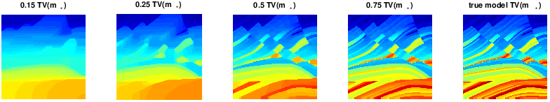
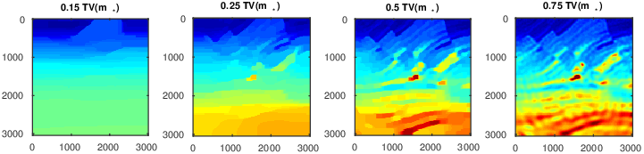
Edge-preserving prior information derives from the premise that the Earth contains sharp edge-like unconformable strata, faults, Salt or Basalt inclusions. Several researchers have worked on ways to promote these edge-like features by including prior information in the form of TV-norms. If performing according to their specification, minimizing the TV-norm of the velocity model \(\mathbf{m}\) on a regular grid with gridpoint spacing \(h\), \[ \begin{equation} \text{TV}(\mathbf{m}) = \frac{1}{h}\sum_{ij}\sqrt{({m}_{i+1,j}-{m}_{i,j})^2 + ({m}_{i,j+1}-m_{i,j})^2}, \label{TV-def} \end{equation} \] acts as applying a multidimensional “velocity blocker”. To make sure that the resulting models remain physically feasible, TV-norm minimization is combined with so-called \(\text{Box}\) constraints that make sure that each gridpoint of the resulting velocity model remains within a user-specified interval—i.e., \(\mathbf{m} \in \text{Box}\) means that \(l \leq m_{i,j} \leq u\) with \(l\) and \(u\) the lower and upper bound respectively. It can be shown, that for a given \(\tau\) \[ \begin{equation} \min_{\mathbf{m}}\|\mathbf{m} - \mathbf{m}_\ast\|^2 \quad\text{subject to}\quad \mathbf{m}\in \text{Box} \text{ and } \text{TV}(\mathbf{m}) \leq \tau, \label{TV-proj} \end{equation} \] finds a unique blocked velocity model that is close to the original velocity model (\(\mathbf{m}_\ast\)) and whose blockiness depends on the size of the TV-norm ball \(\tau\). As the size of this ball increases, the resulting blocked velocity model is less constrained, less blocky, and closer to the original model—juxtapose the TV-norm constrained velocity models in Figure 1 for \(\tau=(0.15,\,0.25,\,0.5,\,0.75,1)\times \tau_{\mathrm{true}}\) with \(\tau_{\mathrm{true}}=\text{TV}(\mathbf{m}_\ast)\). The solution of Equation \(\ref{TV-proj}\) is the projection of the original model onto the intersection of the box- and TV-norm constraint sets. In other words, the solution is the closest model to the input model, but which is within the bounds and has sufficiently small total-variation.

FWI with total-variation like penalties

Edge-preserved regularizations have been attempted by several researchers in crustal-scale FWI. Typically, these attempts derive from minimizing the least-squares misfit between observed (\(\mathbf{d}^\mathrm{obs}\)) and simulated data (\(\mathbf{d}^\mathrm{sim}(\mathbf{m})\)), computed from the current model iterate. Without regularization, the least-squares objective for this problem reads \[ \begin{equation} f(\mathbf{m})=\|\mathbf{d}^\mathrm{obs}-\mathbf{d}^\mathrm{sim}(\mathbf{m})\|^2. \label{objective} \end{equation} \] Now, if we follow the textbooks on geophysical inversion the most straight forward way to regularize the above nonlinear least-squares problem would be to add the following penalty term: \(\alpha \| \mathbf{L}\mathbf{m}\|_2^2\), where \(\mathbf{L}\) represents the identity or a sharpening operator. The parameter \(\alpha\) controls the trade-off between data fit and prior information, residing in the additional penalty term.

Unfortunately, this type of regularization does not fit our purpose because it smoothes the model and does not preserve edges. TV-norms (as defined in Equation \(\ref{TV-def}\)), on the other hand, do preserve edges but are non-differentiable and lack curvature. Both wreak havoc because FWI relies on first- (gradient descent) and second-order (either implicitly or explicitly) derivative information.

As other researchers, including Vogel (2002), Epanomeritakis et al. (2008), Anagaw and Sacchi (2011) and Xiang and Zhang (2016) have done before us, we can seemingly circumvent the issue of non-smoothness altogether by adding a small parameter \(\epsilon^2\) to the definition of the TV-norm in Equation \(\ref{TV-def}\). The expression for this TV-like norm now becomes \[ \begin{equation} \text{TV}_{\epsilon}(\mathbf{m}) = \frac{1}{h}\sum_{ij}\sqrt{(m_{i+1,j}-m_{i,j})^2 + (m_{i,j+1}-m_{i,j})^2 + \epsilon^2} \label{TV-def-smooth} \end{equation} \] and corresponds to “sand papering” the original functional form of the TV-norm at the origin so it becomes differentiable. By virtue of this mathematical property, this modified term can be added to the objective defined in Equation \(\ref{objective}\) — i.e., we have \[ \begin{equation} \min_{\mathbf{m}} f(\mathbf{m})+\alpha \text{TV}_{\epsilon}(\mathbf{m}). \label{def-obj-TV-smooth} \end{equation} \] For relatively simple linear inverse problems this approach has been applied with success (see e.g. Vogel (2002)). However, as we demonstrate in the example below, this behavior unfortunately does not carry over to FWI where the inclusion of this extra tuning parameter \(\epsilon\) becomes problematic.

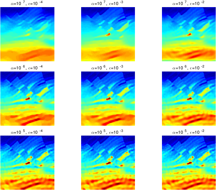
To illustrate this problem, we revisit the subset of the Marmousi model in Figure 1 and invert noisy data generated from this model with a \(10\,\mathrm{Hz}\) Ricker wavelet and with zero mean Gaussian noise added so that \(\|\text{noise}\|_2 / \| \text{signal} \|_2 = 0.25\). Sources and receivers are equally spaced at \(50\,\mathrm{m}\) and we start from an accurate smoothed model. Results of multiple warm-started inversions from \(3\) to \(10\) Herz are shown in Figure 2. Warm-started means we invert the data in \(1\,\mathrm{Hz}\) batches and use the final result of a frequency batch as the initial model for the next batch. In an attempt to mimic relaxation of the constraint as in Figure 1, we decrease the trade-off parameter \(\alpha\in (10^7,\,10^6,\,10^5)\) (rows of Figure 2) and and increase \(\epsilon\in(10^{-4},\,10^{-3},\,10^{-2})\) (plotted in the columns of Figure 2). The latter experiments are designed to illustrate the effects of approximating the ideal TV-norm (\(\text{TV}_{\epsilon}(\mathbf{m})\) for \(\epsilon\rightarrow 0\)).

Even though the inversion results reflect to some degree the expected behavior, namely more blocky for larger \(\alpha\) and smaller \(\epsilon\), the reader would agree that there is no distinctive progression from “blocked” to less blocky as was clearly observed in Figure 1. For instance, the regularized inversion results are no longer edge preserving when the “sandpaper” parameter \(\epsilon\) becomes too large. Unfortunately, this type of unpredictable behavior of regularization is common and exacerbate by more complex nonlinear inversion problems. It is difficult, if not impossible, to predict the inversion’s behavior as a function of the multiple tuning parameters. While underreported, this lack of predictability of penalty-based regularization has frustrated practitioners of this type of total-variation like regularization and explains its limited use so far.

FWI with total-variation norm constraints

Following developments in modern-day optimization (Esser et al., 2016; Esser et al., 2016), we replace the smoothed penalty term in Equation \(\ref{def-obj-TV-smooth}\) by the intersection of box and TV-norm constraints (cf. Equation \(\ref{TV-def}\)), yielding

\[ \begin{equation} \min_\mathbf{m} f(\mathbf{m}) \quad\text{subject to}\quad \mathbf{m}\in \text{Box} \text{ and } \text{TV}(\mathbf{m}) \leq \tau, \label{prob-constr} \end{equation} \] which corresponds to a generalized version of Equation \(\ref{TV-proj}\). Contrary to regularization with smooth penalty terms, minimization problems of the above type do not require smoothness on the constraints. Depending on the objective (data misfit function in our case), these formulations permit different solution strategies. Since the objective of FWI is highly nonlinear and computationally expensive to evaluate, we call for an algorithm design that meets the following design criteria:

• each model update depends only the current model and gradient and does not require additional expensive gradient and objective calculations;

• the updated models satisfy all constraints after each iteration;

• arbitrary number of constraints can be handled as long as their intersection is non-empty;

• manual tuning of parameters is limited to a bare minimum.

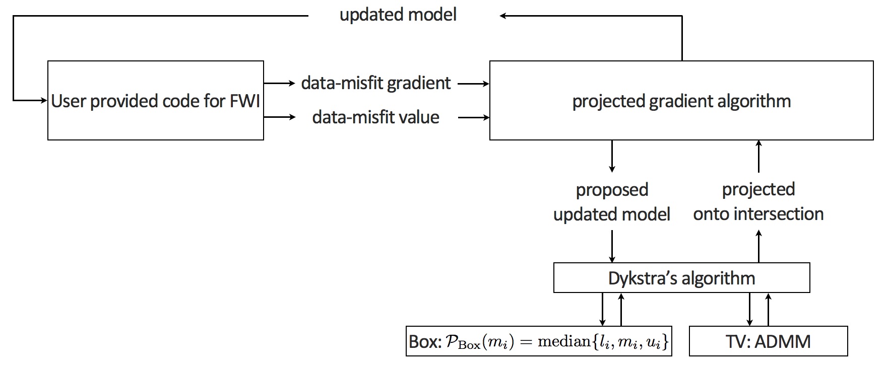
While there are several candidate algorithms that meet these criteria, we consider a projected-gradient method where at the \(k^{\text{th}}\) iteration the model is first updated by the gradient, to bring the data residual down, followed by a projection onto the constraint set \(\mathcal{C}\). The projection onto the set \(\mathcal{C}\) is denoted by \(\mathcal{P}_{\mathcal{C}}\). The main iteration of the projected gradient algorithm is therefore given by \[ \begin{equation} \mathbf{m}_{k+1}=\mathcal{P}_{\mathcal{C}} (\mathbf{m}_k - \nabla_{\mathbf{m}}f(\mathbf{m}_k)). \label{proj_grad_step} \end{equation} \] After this projection, each model is guaranteed to lie within the intersection of the \(\text{Box}\) and TV-norm constraints—i.e., \(\mathcal{C}=\{\mathbf{m}:\,\mathbf{m}\in \text{Box} \text{ and } \text{TV}(\mathbf{m}) \leq \tau\}\). During the projections defined in Equation \(\ref{TV-proj}\), the resulting model (\(\mathbf{m}_{k+1}\)) is unique while it also stays as close as possible to the model after it has been updated by the gradient.

While conceptually easily stated, uniquely projecting models onto multiple constraints can be challenging especially if the individual projections do not permit closed-form solutions as is the case with the TV-norm. For our specific problem, we use Dykstra’s algorithm (Boyle and Dykstra, 1986) by alternating between projections onto the \(\text{Box}\) constraint and onto the TV-norm constraint. Projecting onto an intersection of constraint sets is equivalent to running Dykstra’s algorithm: \(\mathcal{P}_{\mathcal{C}} (\mathbf{m}_k - \nabla_{\mathbf{m}}f(\mathbf{m}_k)) \Leftrightarrow \text{DYKSTRA}(\mathbf{m}_k - \nabla_{\mathbf{m}}f(\mathbf{m}_k))\).

The projection onto the box constraint is provided in closed-form, by taking the elementwise median. The projection onto the set of models with sufficiently small TV is computed via the Alternating Direction Method of Multipliers (ADMM, Boyd et al. (2011)). Dykstra’s algorithm and ADMM are both free of tuning parameters in practice. The \(three\) steps above can be put in one nested-optimization workflow, displayed in Figure 3.

Dykstra’s algorithm for the projection onto the intersection of constraints was first proposed by Smithyman et al. (2015) in the context of FWI and can be seen as an alternative approach to the method proposed by the late Ernie Esser and that has resulted in major breakthroughs in automatic salt flooding with TV-norm and hinge-loss constraints (Esser et al., 2016; Esser et al., 2016).

Why constraints?

Before presenting a more elaborate example of constrained FWI on Salt plays, let us first discuss why constrained optimization approaches with projections onto intersections of constraint sets are arguably simpler to use than some other well known regularization techniques.

• Constraints translate prior information and assumptions about the geology more directly than penalties. Although the constrained formulation does not require the selection of a penalty parameter, the user still needs to specify parameters for each constraint. For Equation \(\ref{prob-constr}\), this is the size of the TV ball \(\tau\). However, compared to trade-off parameter \(\alpha\), the \(\tau\) is directly measurable from a starting or any other model that serves as a proxy.

• Absence of user-specified weights. Where regularization via penalty terms relies on the user to provide weights for each penalty term, unique projections onto multiple constraints can be computed with Dykstra’s algorithm as long as these intersections are not empty. Moreover, the inclusion of the constraints does not alter the objective (data misfit) but rather it controls the region of \(f(\mathbf{m})\) that our non-linear data fitting procedure is allowed to explore. This is especially important when there are many (\(\geq 2\)) constraints. For standard regularization, it would be difficult to select the weights because the different added penalties are all competing to bring down the total objective.

• Constraints are only activated when necessary. Before starting the inversion, it is typically unknown how ‘much’ regularization is required, as this depends on the noise level, type of noise, number of sources and receivers as well as the medium itself. The advantage of projection methods for constrained optimization is that they only activate the constraints when required. If a proposed model, \(\mathbf{m}_k - \nabla_{\mathbf{m}}f(\mathbf{m}_k)\), satisfies all constraints, the projection step does not do anything. The data-fitting and constraint handling are uncoupled in that sense. Penalty methods, on the other hand, modify the objective function and will for this reason always have an effect on the inversion.

• Constraints are satisfied at each iteration. We obtained this important property by construction of our projected-gradient algorithm. Penalty methods, on the other hand, do not necessarily satisfy the constraints at each iteration and this can make them prone to local minima.

Objective and gradients for two waveform inversion methods

To illustrate the fact that the constrained approach to waveform inversion does not depend on the specifics of a particular waveform inversion method (we only need a differentiable \(f(\mathbf{m})\) and the corresponding gradient \(\nabla_\mathbf{m} f(\mathbf{m})\)), we briefly describe the objective and gradient for full-waveform inversion (FWI) and Wavefield Reconstruction Inversion (WRI, Leeuwen and Herrmann (2013)). These two methods will be used in the results section. We would like to emphasize that we do not need gradients of the constraints or anything related to the constraints. Only the projection onto the constraint set is necessary. For derivations of these gradients, see e.g., Plessix (2006) for FWI and Leeuwen and Herrmann (2013) for WRI.

	FWI	WRI
Objective:	\(f(\mathbf{m})=\frac{1}{2}\| P \mathbf{u}- \mathbf{d}^\mathrm{obs}\|^{2}_{2}\)	\(f(\mathbf{m}) = \frac{1}{2}\| P \mathbf{\bar{u}} - \mathbf{d}^\mathrm{obs}\|^{2}_{2} +\frac{\lambda^2}{2}\|A(\mathbf{m}) \mathbf{\bar{u}} -\mathbf{q}\| ^{2}_{2}\)
Field:	\(\mathbf{u}=A^{-1} \mathbf{q}\)	\(\mathbf{\bar{u}} = (\lambda^2 A(\mathbf{m})^* A(\mathbf{m}) + P^* P)^{-1} (\lambda^2 A(\mathbf{m})^* \mathbf{q} + P^* \mathbf{d}^\mathrm{obs})\)
Adjoint:	\(\mathbf{v}=-A^{-*} P^*(P \mathbf{u}- \mathbf{d}^\mathrm{obs})\)	none
Gradient:	\(\nabla_{\mathbf{m}}f(\mathbf{m}) =G(\mathbf{m},\mathbf{u})^* \mathbf{v}\)	\(\nabla_{\mathbf{m}} f(\mathbf{m}) = \lambda^2 G(\mathbf{m},\mathbf{\bar{u}})^* \big( A(\mathbf{m})\mathbf{\bar{u}} -\mathbf{q} \big)\)
Partial derivative:	\(G(\mathbf{m},\mathbf{u})={\partial A (\mathbf{m}) \mathbf{u}} / {\partial \mathbf{m}}\)	\(G(\mathbf{m},\mathbf{u})={\partial A (\mathbf{m}) \mathbf{\bar{u}}} / {\partial \mathbf{m}}\)

Results

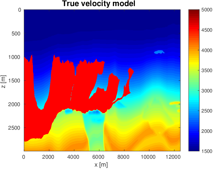
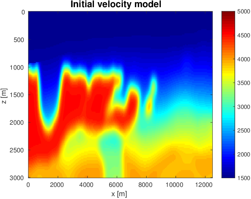
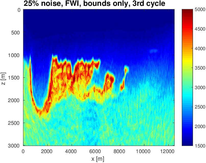
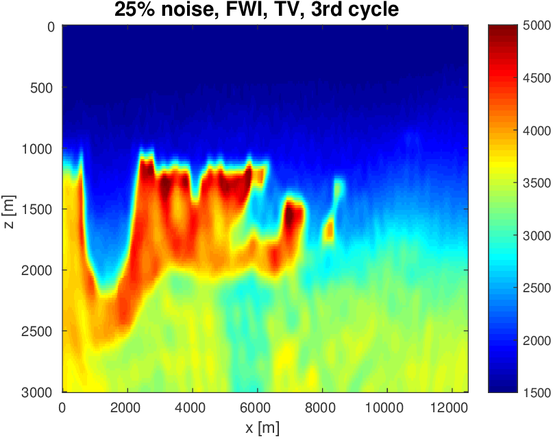
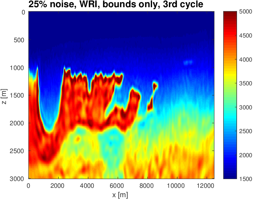
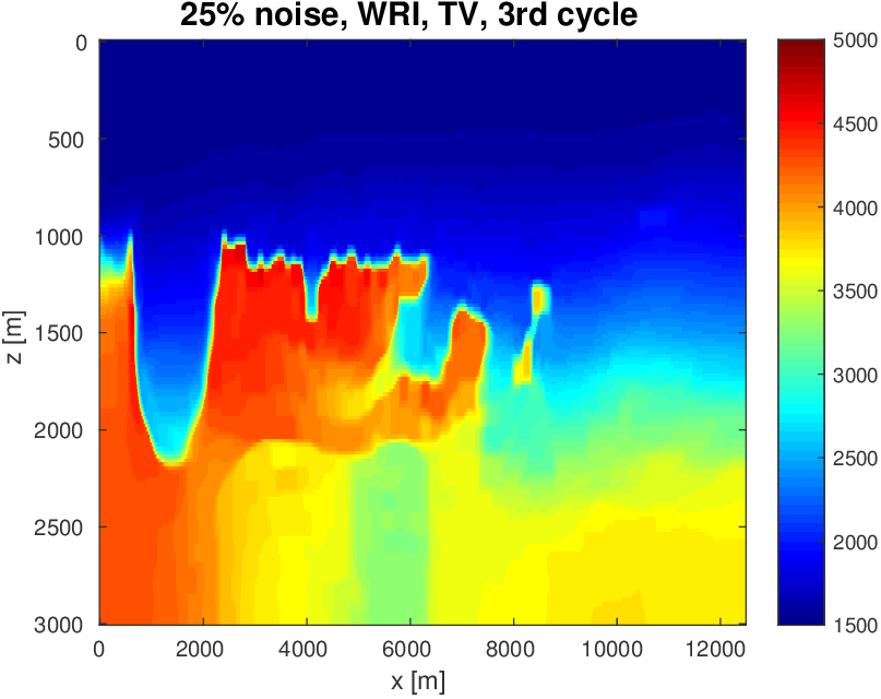
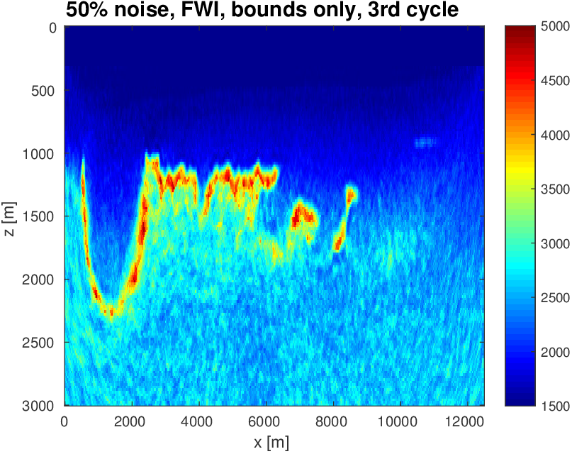
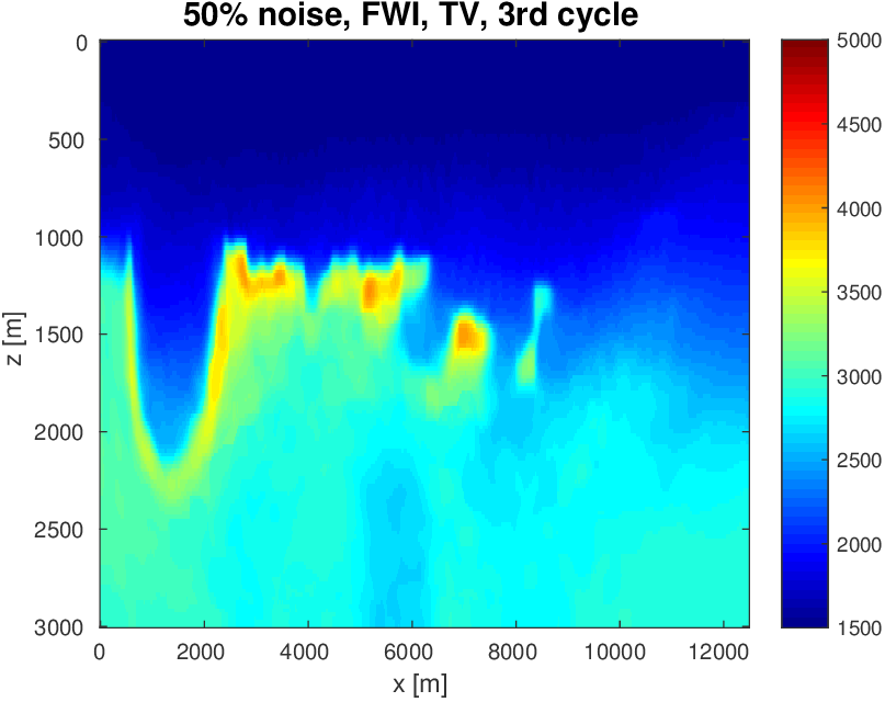
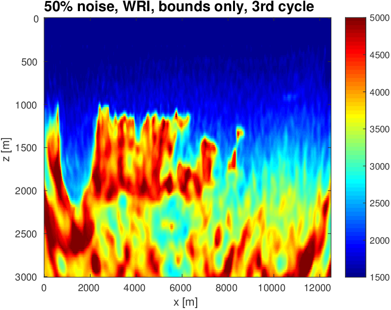
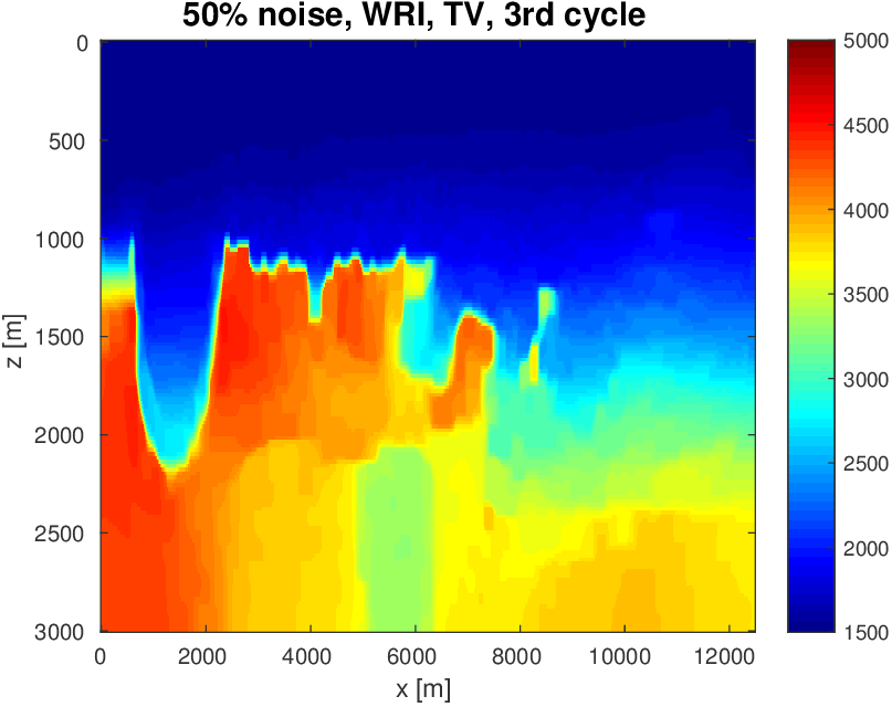
To evaluate the performance of our constrained waveform-inversion methodology, we present the West part of the BP 2004 velocity model (Billette and Brandsberg-Dahl, 2005), Figure 5. The inversion strategy uses simultaneous sources and noisy data. We present results for two different waveform inversion methods and two different noise levels. As we can clearly see from Figures 6 and 7, FWI with bound constraints (\(l=1475\,\mathrm{m/s}\) and \(u=5000\,\mathrm{m/s}\)) only is insufficient to steer FWI in the correct direction despite the fact we used a reasonably accurate starting model (Figure 5b) by smoothing the true velocity model (Figure 5a). WRI with bound constraint only does better, but the results are still unsatisfactory. The results obtained by including TV-norm constraints, on the other hand, lead to a significant improvement and sharpening of the Salt.

We arrived at this result via a practical workflow where we select the \(\tau = \text{TV}(\mathbf{m}_0)\), such that the initial model (\(\mathbf{m}_0\)) satisfies the constraints. We run our inversions with the well-established multiscale frequency continuation strategy keeping the value of \(\tau\) fixed. Next, we rerun the inversion with the same multiscale technique, but this time with a slightly larger \(\tau\), such that more details can enter into the solution. We select \(\tau= 1.25 \times \text{TV}(\mathbf{m}_1)\), where \(\mathbf{m}_1\) is the inversion result from the first inversion. This is repeated one more time, so we run the inversions three times, each run uses a different constraint. For comparison (juxtapose Figures 6a and 6b) , we do the same for the inversions with the box constraints except in that case we do not impose the TV-norm constraint and keep the box constraints fixed.

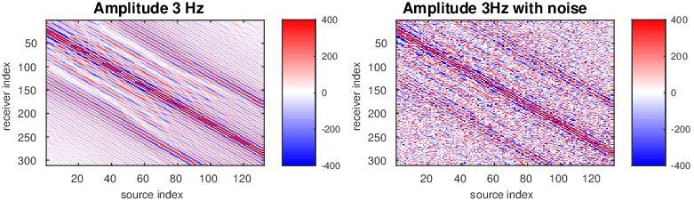
As before, our inversions are carried out over multiple frequency batches with a time-harmonic solver for the Helmholtz equation and for data generated with a 15Hz Ricker wavelet. The inversions start at 3 Hertz and run up to 9 Hertz. The data contains noise, so that measured over all frequencies, the noise to signal ratio is \(\|\text{noise}\|_2 / \| \text{signal} \|_2 = 0.25\) for the first example and \(\|\text{noise}\|_2 / \| \text{signal} \|_2 = 0.50\) for the second example. This means that the 3 Hertz data is noisier than frequencies closer to the peak frequency. Frequency domain amplitude data is shown in Figure 8 for the starting frequency. The starting model is kinematically correct because it is a smoothed version of the true model (cf. Figure 5a and 5b). The model size is about 3 km by 12 km, discretized on a regular grid with a gridpoint spacing of 20 meters.

The main goal of this experiment is to delineate the top and bottom of the salt body, while working with noisy data and only \(8\) (out of 132 sequential sources) simultaneous sources redrawn independently after each gradient calculation. The simultaneous sources activate every source at once, with a Gaussian weight. The distance between sources is \(80\) meters while the receivers are spaced \(40\) meters apart.

As we can see, limiting the total-variation norm serves two purposes. (i) We keep the model physically realistic by projecting out highly oscillatory and patchy components appearing in the inversion result where the TV-norm is not constrained. These artifacts are caused by noise, source crosstalk and by missing low frequencies and long offsets that lead to a non-trivial null space easily inhabited by incoherent velocity structures that hit the bounds. (ii) We prevent otherwise ringing artifacts just below and just above the transition into the Salt. These are typical artifacts caused by the inability of regular FWI to handle large velocity contrasts. Because the artifacts increase the total-variation by a large amount, limiting the total-variation norm mitigates this well-known problem to a reasonable degree.

The noisy data, together with the use of \(8\) simultaneous sources effectively creates “noisy” gradients because of the source crosstalk. Therefore, our projected gradient algorithm can be interpreted as “denoising” where we map at each iteration incoherent energy onto coherent velocity structure. For this reason, the results with TV-norm constraints are drastically improved compared to the inversions carried out with bound constraints only. The inability of bounds constrained FWI to produce reasonable results for FWI with source encoding was also observed by Esser et al. (2015) (see his Figure 19). While removing the bounds could possibly avoid some of these artifacts from building up, it would lead to physically unfeasible low and high velocities, which is something we would need to avoid at all times.

Again when the TV-norm and box constraints are applied in tandem, the results are very different. Artifacts related to velocity clipping no longer occur because they are removed by the TV-norm constraint while the inclusion of this constraint also allows us to improve the delineation of top/bottom Salt and the Salt flanks. The results also show that WRI, by virtue of including the wavefields as unknowns, is more resilient to noise and local minima compared to FWI and that WRI obtains a better delineation of the top and bottom of the Salt structure.

Discussion and summary

Our purpose was to demonstrate the advantages of including (non-smooth) constraints over adding penalties in full-waveform inversion (FWI). While this text is certainly not intended to extensively discuss subtle technical details on how to incorporate non-smooth edge-preserving constraints in full-waveform inversion, we explained the somewhat limited success of including total-variation (TV) norms into FWI. By means of stylized examples, we revealed an undesired lack of predictability of the inversion results as a function of the trade-off and smoothing parameters when we include TV-norm regularization as an added penalty term. We also made the point that many of the issues of including multiple pieces of prior information can be overcome when included as intersections of constraints rather than as the sum of several weighted penalties. In this way, we were able to incorporate the edge-preserving TV-norm and Box constraints controlling the spatial variations as well as the permissible range of inverted velocities with one parameter aside from the lower and upper bounds for the seismic velocity. As the stylized examples illustrate, this TV-norm parameter predictably controls the degree blockiness of the inverted velocity models making it suitable for FWI on complex models with sharp boundaries.

Even though the Salt body example we presented is synthetic and inverted acoustically with the “inversion crime”, it clearly illustrates the important role properly chosen constraints can play when combined with search extensions such as Wavefield Reconstruction Inversion (WRI). Without TV-norm constraints, artifacts stemming from source crosstalk, noise and from undesired fluctuations when moving in and out of the Salt overcome FWI because the inverted velocities hit the upper and lower bounds too often. If we include the TV-norm, this effect is removed and we end up with a significantly improved inversion result with clearly delineated Salt. This example also illustrates that the constrained optimization approach applies to any waveform inversion method. Results are presented for FWI and WRI, where WRI results delineate the Salt structure better and exhibit more robustness to noise.

Acknowledgements

This work was financially supported in part by the Natural Sciences and Engineering Research Council of Canada Collaborative Research and Development Grant DNOISE II (CDRP J 375142-08). This research was carried out as part of the SINBAD II project with the support of the member organizations of the SINBAD Consortium.

We would like to thank our former colleague Ernie Esser (1980-2015) for numerous discussions about constrained optimization and splitting methods during the fall of 2014.