 of research program at UBC to tackle wave-equation based inversion, imaging, and related problems._](./Fig/mindmap.png)
Mind map of research program at UBC to tackle wave-equation based inversion, imaging, and related problems.
Felix J. Herrmann1, Andrew J. Calvert2, Ian Hanlon3, Mostafa Javanmehri4, Rajiv Kumar5, Tristan van Leeuwen6, Xiang Li7, Brendan Smithyman8, Eric Takam Takougang9, and Haneet Wason10
As conventional oil and gas fields are maturing, our profession is challenged to come up with the next-generation of more and more sophisticated exploration tools. In exploration seismology this trend has led to the emergence of wave-equation based inversion technologies such as reverse-time migration and full-waveform inversion. While significant progress has been made in wave-equation based inversion, major challenges remain in the development of robust and computationally feasible workflows that give reliable results in geophysically challenging areas that may include ultra-low shear velocity zones or high-velocity salt. Moreover, sub-salt production carries risks that needs mitigation, which raises the bar from creating sub-salt images to inverting for sub-salt overpressure.
Amongst the many challenges that wave-equation based inversion faces—see the mind map in Figure mindmap outlining our research program at UBC—we focus in this contribution on reducing the excessive computational costs of full-waveform inversion (FWI). We accomplish these cost reductions by using modern techniques from machine learning and compressive sensing. Contrary to many implementations of wave-equation based inversion, we propose a methodology where we do not insist on using all data—i.e., looping over all sources, to calculate the velocity model updates. Instead, we rely on a formulation that only calls for more data and more accuracy in the wave simulations as needed by the inversion. This leads to major savings in particular in the beginning when we are far from the solution. Since this approach reduces the computational costs significantly, we open the way to test different scenarios or to include more sophisticated regularization. Without this cost reduction, these would both be computationally infeasible.
The paper is organized as follows. First, we introduce the basics of full-waveform inversion, followed by stochastic sampling techniques to reduce the computational costs. Next, we propose an adaptive scheme that selects the required sample size–i.e, the number of source experiments that partake in the inversion, and forward modeling accuracy. Recent results on the Chevron Gulf of Mexico dataset are discussed next followed by a discussion on challenges of FWI and possible roads ahead.
Full-waveform inversion (FWI) is a parameter estimation problem, seeking earth models that explain observed data typically collected in shot records. FWI is generally cast as an optimization problem where earth models are found by minimizing the misfit between observed and simulated data—i.e, we solve the following optimization problem:
\[\min_{\mathbf{m}}\,\Phi(\mathbf{m})=\sum_{i=1}^M\frac{1}{2}\|\mathbf{d}^{\text{obs}}_{i}-\mathbf{d}^{\text{syn}}_{i}(\mathbf{m})\|_2^2\quad\text{where}\quad\mathbf{d}_i^{\text{syn}}(\mathbf{m})=\mathbf{P}_i\mathbf{A}_i(\mathbf{m})^{-1}\mathbf{q}_i,\]
where
Solutions of the above minimization problem are typically found by using iterative optimization techniques, which use local derivative information to compute descent directions that minimizes the objective \(\Phi(\mathbf{m})\). At the bare minimum, these optmizations consist of the following four steps for each experiment (Tarantola and Valette 1982; Plessix 2006): (i) data prediction by solving the wave-equation by inverting \(\mathbf{A}_i(\mathbf{m})\), (ii) calculation of the misfit between observed and predicted data, (iii) solution of the time-reversed or adjoint wave-equation using the data-residual as the source-term, (iv) calculation of the model updates by correlating the forward and adjoint wavefields for each experiment, followed by a summation over the experiments yielding the gradient, and (v) computing the model update by properly scaling the gradient—e.g., by conducting a line search and approximately inverting the Hessian. This leads to efficient algorithms because the steps before the summation can be carried out in parallel.
While the above procedure is largely responsible for current successes of full-waveform inversion to field data, numerous challenges remain. These include
Numerous researchers have embarked on addressing these challenges. Since successful application of geophysical methods often depends on multiple runs to fine-tune a multitude of inversion parameters, our aim in this paper is to (i) speedup turnaround times and (ii) to automate the inversion as much as possible. We accomplish this by casting FWI as a optimization problem that is economic in the amount of data (number of sources) and accuracy of wave-equation solves it needs in the early stages of the inversion. In this way, we make FWI computationally manageable so resources can be spend on where it matters namely in figuring out parameter settings, (pre)-processing, and starting model sensitivities.
Essentially, our approach is based on the intuitive premise that data misfit and gradient calculations do not need to be accurate at the beginning of an iterative optimization scheme when the model explains the data poorly. We translate this idea to a concrete and practical algorithm where we control the errors by adaptively increasing the number and shots and simulation accuracy.
Aside from lack of robustness with respect to starting models and its ability to capture the wave physics adequately, FWI has been challenging computationally because the total work needed to calculate model updates scales linearly with the number of source experiments. To make matters worse, the number of source experiments and amount of work per experiment increase exponentially with the survey area. For that reason, we face with 3D FWI similar problems as researchers in supervised machine learning face, who are confronted with exponential growth in “big data”. Fortunately, researchers in both fields have been able to exploit the separable structure of their problems, namely the objective function and its gradient have in both fields the form of a sum over different experiments. Following recent work by (Aravkin et al. 2012), this sum can be interpreted as an average over the experiments that can be approximated by its sample average—i.e, we have
\[\Phi(\mathbf{m})\approx\frac{1}{M}\sum_{i\in\mathcal{I}}{\phi_i}(\mathbf{m};\mathbf{d}^{\text{obs}}_{i},\mathbf{d}^{\text{syn}}_{i})\quad \text{and}\quad \mathbf{g}:=\nabla\Phi(\mathbf{m})\approx\frac{1}{M}\sum_{i\in\mathcal{I}}{\nabla\phi_i(\mathbf{m};\mathbf{d}^{\text{obs}}_{i},\mathbf{d}^{\text{syn}}_{i})},\]
where the sum now runs only over a subset of experiments \(\mathcal{I}\) with \(\#\,\text{of elements}\{\mathcal{I}\}\ll M\). While this reduction in the sample size, i.e., the number of experiments, leads to a reduction in the computational costs, practical application of this approach calls for an answer of the following questions:
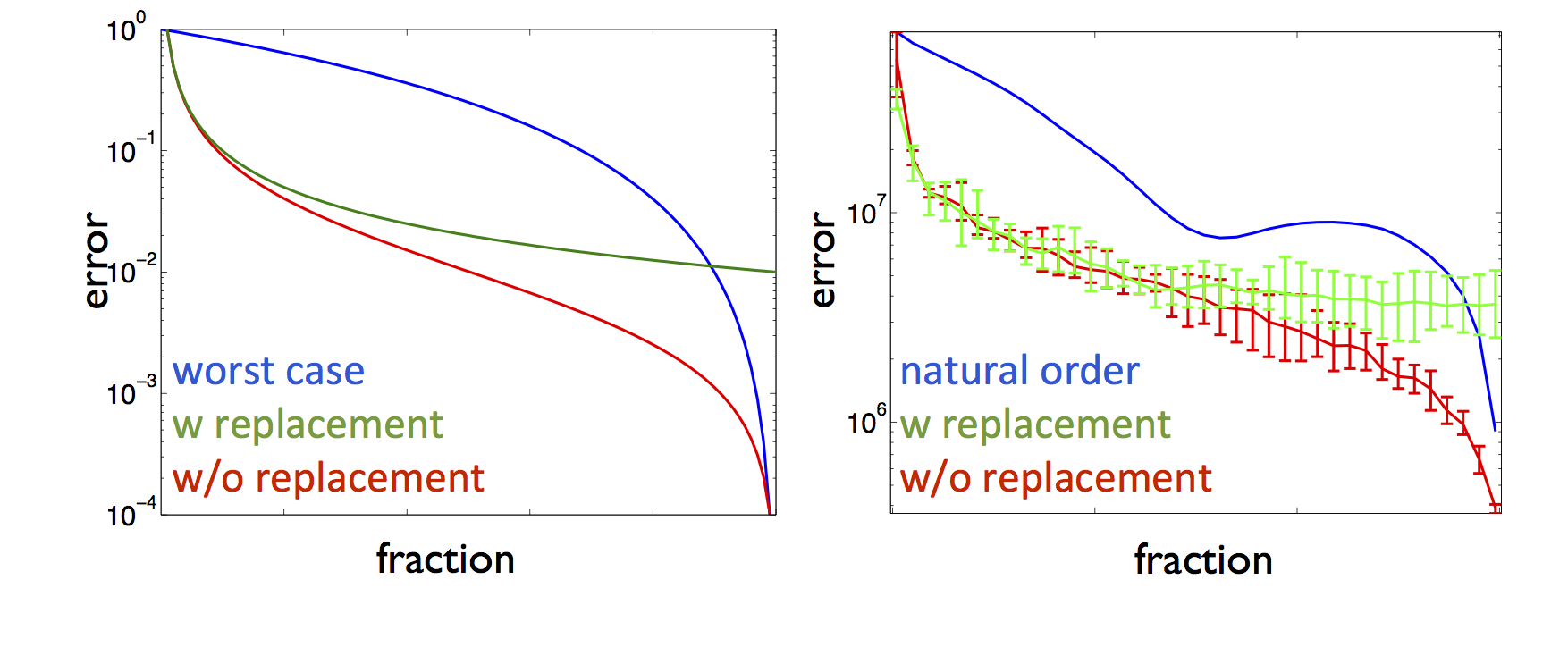
what error do we make when we only work with subsets of experiments and how does this error behave as a function of the size of these subsets?
how should we select these subsets at each iteration of the optimization to assure convergence and to minimize subsampling-related errors accumulated during the optimization?
Substantial theoretical progress has been made towards answering these questions (see e.g. Friedlander and Schmidt (2012),Aravkin et al. (2012)) . In the next sections, we summarize and translate these findings as they relate to the practicalities of FWI.
The first step in the reduction of the computational costs of FWI is selection of subsets of source experiments. Selection of these subsets leads to errors and Figure error shows the behavior of the theoretical and empirical sampling errors of the gradient as a function of sample size divided by the total data size. In this plot, we compare the worst case scenario, where we sample the least informative experiments, with randomized sampling with and without replacement. As expected, the sampling errors for the randomized sampling decay as the fraction increases but this decay stalls if we allow the experiments to be selected more than once. This is the case when we select the source experiments with replacement11. However, if we select the experiments without replacement the error continues to decay and the sampling eventually becomes deterministic as the fraction of selected sources goes to one. These theoretical predictions are confirmed by empirical findings also included in Figure error. These findings also show that we can control the error of each gradients but the question “how does this subsampling error affects the convergence of FWI?” still needs to be answered. The field of stochastic optimization attempts to answer this question.
Even through randomly choosing small subsets of sources speeds up computations, it introduces unwanted random errors in the misfit and gradient calculations that may affect convergence of FWI and the quality of the end result. By choosing independent random subsets for each gradient calculation—an approach known as stochastic gradient descent widely used in data-intensive fields such as machine learning—convergence can be greatly improved because biases in the errors in the gradient are removed.
While independent renewals of the source subsets certainly leads to a speedup of the convergence of the algorithm, choosing these subsets continues to introduce random errors into the optimization, which eventually stalls progress of the algorithm, in particular when there is noise (see e.g. Krebs et al. (2009) and van Leeuwen, Aravkin, and Herrmann (2011)). So the question arises how to choose a dynamic sampling strategy that mitigates the effect of these sampling errors by growing the sample size such that the algorithm continues to converge. Recent theoretical analysis by Friedlander and Schmidt (2012) and Aravkin et al. (2012) shows that this can be accomplished by increasing the sample size fast enough so that the sampling error decays at least as fast as the inversion makes progress towards the solution. Even though this approach sounds intuitive—why would one need an accurate gradient if one is still far from the solution—it can lead to a somewhat counter intuitive sampling strategy where sample-sizes will be chosen to increase only slowly in situations where the optimization converges slowly, e.g. in cases where the problem is ill-posed.
As Figure samplingbg indicates, significant speedups in the turnaround time of FWI is achievable if we follow the above sampling strategy. However, this ten-fold speed up was obtained in a somewhat ad hoc manner because the convergence rate of FWI is generally not known beforehand and that in turn means that we do not know how to increase the sample size. To address this practical issue, we introduce in the next section a heuristic algorithm that allows us to control errors related to subsampling and forward modeling accuracy adaptively.

Aside from the number of source experiments—whether these are the number of shots or the number of frequencies of a time-harmonic wave-equation simulator—the cost of wave-equation solves depends on the desired accuracy. By the same token of controlling errors in the sample mean, by increasing the sample size, we can also choose to increase the accuracy of wave-equation solves as needed by the optimization. For indirect wave-equation solvers, whose accuracy depends on the number of iterations, this leads to additional savings during the early stages of the inversion where accuracy is not yet needed. However, as before, we will need to control these errors to guarantee convergence. For this purpose, we first show how to calculate the misfit and gradient with selected tolerance.
A key component of our stochastic optimization scheme for FWI are the approximate misfit and gradient calculations with a prescribed but beforehand unknown tolerance. To this end, we introduce a heuristic method that calculates this tolerance since we do not know the true error in the modeling because we do not have access to the true forward modelled result. Instead, we use an iterative procedure (outlined below or see van Leeuwen and Herrmann (2013) for further detail) that finds the smallest \(k\) for which
\[ \left|\phi_i(\mathbf{m},\alpha^k\epsilon) - \phi_i(\mathbf{m},\alpha^{k+1}\epsilon)\right| \leq \eta \phi_i(\mathbf{m},\alpha^{k+1}\epsilon)\quad i\in \mathcal{I},\]
for some \(0<\alpha<1\), and for a user defined \(\eta\) and initial tolerance of \(\epsilon=10^{-2}\). During the \(k^{th}\) iteration (with \(k=1\cdots 10\)) of this procedure, we solve the wave-equation up to \(\epsilon\) and we compute the two-norm of the data residual—i.e., the two-norm of the difference between the forward modeled and observed data. If the absolute value of the difference between the norms of the current and previous residual is smaller then an \(\eta\) fraction of the current residual, we are done. Otherwise, we multiply the tolerance \(\epsilon\) with \(\alpha\) and continue the iterative wave-equation solve with a warm start to reach this new tolerance. We continue to lower the tolerance until the improvement in the residual norm falls below a certain fraction (\(\eta\)) of the residual norm of the current iteration. Given this empirically found tolerance \(\epsilon\), we calculate the adjoint wavefield, the misfit, and the gradient.
The advantage of this approach is that it solves the forward and adjoint wavefields to an accuracy commensurate with the data misfit—i.e., the norm of the residual. This means that initially, we do not solve the wave-equation accurately since the residual is still large at that point because we are still far away from the solution of the FWI problem. As we converge towards the solution, we increase the accuracy and we do this only when we bring the residue down. In this way, we end up with a highly economic approach to FWI, which we summarize in the matlab pseudo code for a single source experiment below.
function [phi,g] =  misfit(m,eta)
% Initialization
phi = 0,  g = zeros(N,1);  epsilon = 0.01; alpha = 0.5; r(1) = 0;
for k = 2 : 10
% Solve forward equation to epsilon accuracy
    u = HelmholtzSolve(A(m),s,epsilon);
% compute norm residual
    r(k) = norm(P*u - d_obs)
% check residual
    if abs(r(k) - r(k-1)) <= eta r(k)
        break;
    else
        epsilon = alpha*epsilon
    endif
end
% solve adjoint equation
    v = HelmholtzSolve(A(m)',P'*(P*u-d_obs),epsilon);
% compute misfit and gradient
    phi = phi + norm(P*u - d_obs);
    g    = g   + omega^2*u'.*v;
end
MATLAB pseudo code for approximate misfit and gradient calculations.
With the approximate misfit and gradient calculations in place, we our now in a position to put the overal optimization scheme together. For this we need to come up with a scheme that selects the sample size and \(\eta\) parameter, which measures the fraction to within which we want to reduce the two norm of the residu. We start the procedure by setting the sample size and fraction to some initial value, e.g., \(b=1\) and \(\eta=1\), followed by the computation of the misfit function for the starting model \({\mathbf{m}}_0\) and for \(b\) randomly selected source(s). Next, we use the approximated misfit and gradient to compute a linesearch to calculate the correct scaling. If this linesearch is not successful, we reduce the fraction \(\eta\) by a factor of two—i.e., \(\eta\mapsto \eta/2\). This forces the misfit and gradient to be calculated more accurately. We repeat this procedure until the linesearch becomes successful. At that point, we draw a new subset of random shots and calculate the misfit and gradient for this misfit. Next, we compute the average of the misfits for these two independent subsets and compare this average with the average misfit of the previous iteration. If the average misfit of the current iteration is larger or equal to the average of the previous iteration, we increase the sample size by one (until we reach the total number of source experiments \(M\)). Otherwise, we compute a linesearch on the last subset and update the model. We repeat this procedure until a maximal number of outer iterations is reached or until the data is fit within some user defined tolerance. The described procedure is summarized in the matlab pseudo code below.
% Initialize eta = 0.1; b = 1;beta = 1; bmax = M;
% Choose subset of sources
locs = randperm(1:M); I_0 = locs(1:b);
% Evaluate misfit and gradient at initial guess
[phi_0,g_0] = misfit(m_0,I_0,eta);
while  not converged
% Linesearch
   [m_k+1,phi_k+1,g_k+1}] = linesearch(phi_k,g_k);
   if linesearch successful
% Draw new independent subset of sources
      locs = randperm(1:M); I_k+1 = locs(1:b);
% Compute misfit and gradient for new sample
      [psi_prime_k+1,g_prime__k+1] = misfit(m_k+1, I_k+1,eta);
% Check average descent
      if (psi_k+1 + psi_prime_k+1) >= (psi_k + psi_prime_k);
         b = min(b + beta, b_max);
      end;
   psi_k+1 = psi_prime_k+1;
   g_k+1   = g_prime_k+1;
   k = k + 1;
   else
      eta = eta/2;
   end;
end
Pseudo code for the stochastic FWI with sample size and wave-equation accuracy selection.
After each iteration, if the linesearch is successful we draw a new independent subset of sources and we check for average descent amongst the previous and new source subset selection. If the average misfit does not decrease, the algorithm increases the sample size by \(\beta\). For a failing linesearch, the algorithm calls for more accuracy for the misfit and gradient calculations by decreasing \(\eta\mapsto \eta/2\). As a consequence, the algorithm is economic in its use of computational resources because it only calls for data and more accuracy when needed.
This stochastic approach with sample size and accuracy selection is in sharp contrast with most existing optimization strategies employed by industry that typically insist on working with all data at full accuracy. Amongst existing economic approaches, there is the fast method with source encoding, advocated by (Krebs et al. 2009) and later by (van Leeuwen, Aravkin, and Herrmann 2011,), which offer no or practically limited guarantees of convergence. We overcome this problem by controlling the error by increasing the accuracy and sample size as needed. Before discussing, our latest results on a complex 2D synthetic for the Gulf of Mexico using a similar approach, let us first briefly evaluate the performance of our algorithm on a small 3D synthetic.
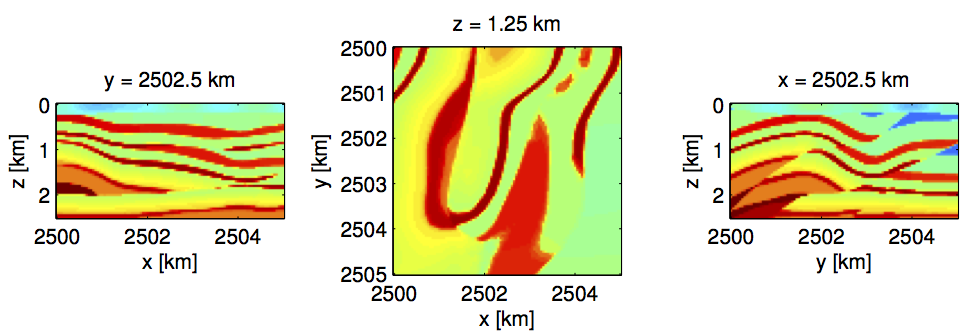
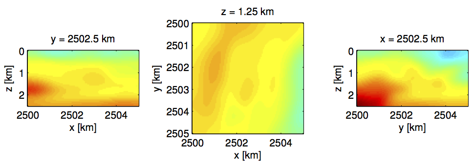
To demonstrate the performance of our proposed frugal approach to FWI, we invert data generated with iWave, an open-source time-domain finite-difference code (Terentyev et al.), for a \(5 \,\mathrm{km} \times\,5 \,\mathrm{km}\) central part of a well-known benchmark model for seismic inversion (the Overthrust model) with \(50 \,\mathrm{m}\) spacing. The true and initial models for this small example are plotted in Figure overtr_v and overtr_v0, respectively. The data was collected for a total of only 121 sources and 2601 receivers (both regularly spaced).
The inversions are carried out by the above described algorithms implemented in (parallel) Matlab, with the exception of our row-based preconditioner (Leeuwen et al. 2012,), which is implemented in C and is called from Matlab using a MEX interface. During the inversion, we use three frequencies \(f=4,6,8\) Hz and adapt the gridspacing to ensure a minimum of 10 gridpoints per wavelength. All experiments were conducted on a small Dual-Core SuperMicro system with 2 Intel(R) Xeon(R) CPU E5-2670 0 @ 2.60GHz and with 128 GB RAM.
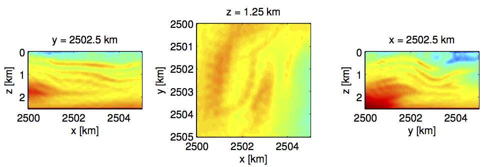
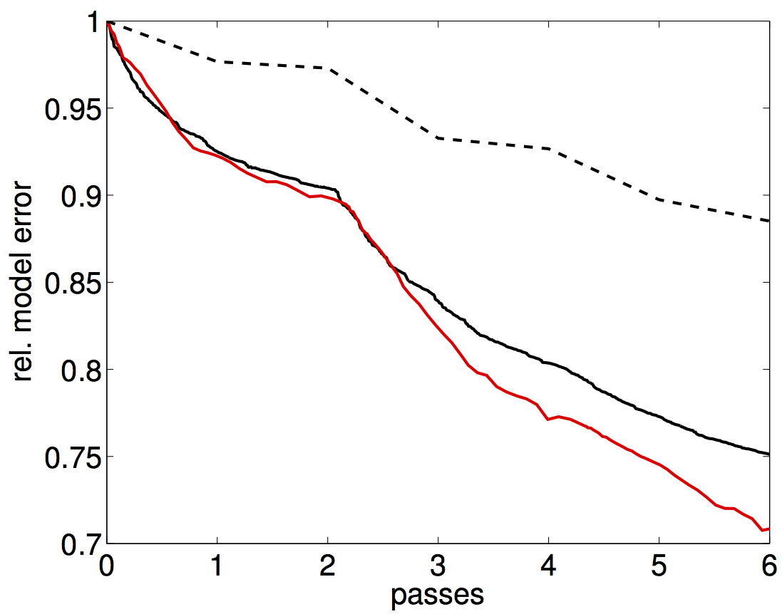
To mimic actual real-live situations, where computational resources and turn-around times are contraints, we limit the total passes through the data per frequency to only two and compare the results following three scenarios, namely, (i) work with one shot at the time \((b=1)\), (ii) work with all shots \((b=121)\), or (iii) choose the number of shots adaptively. In all cases, we select the accuracy of the simulations as needed. While the amount of work in these three scenarios is the same, we would expect the results for the first and third method to be superior compared to the scenario where we insist to work with all data for each misfit and gradient calculation. Indeed Figure vovertr_b121_f and vovertr_binc_f confirm this prediction and shows a drastic improvement in the inversion results where we work subsets of the data only. This improvement is also reflected in the plots for the relative model error, which we included in Figure error_overtr2. These plots show that working with subsets pays when one only has access to a limited computational budget. While the improvement of the our adaptive method may not be drastic in this example, there are guarantees that this method will actually converge.

Aside from reducing demands on computational resources, the presented randomized source subsampling technique also creates the possibility to use sophisticated regularization techniques to stabilize FWI for complex geological areas and for situations where the simulations do not totally capture the physics of the problem, e.g. by inverting elastic data using a scalar velocity-only acoustic code. The Chevron Gulf of Mexico dataset is an example of such a situation where the presence of salt and elastic phases; lack of long offsets; poor signal to noise at low frequencies, all make this a very challenging dataset for acoustic only FWI. To overcome these realistic, but for FWI highly disadvantageous circumstances, we developed the following workflow:
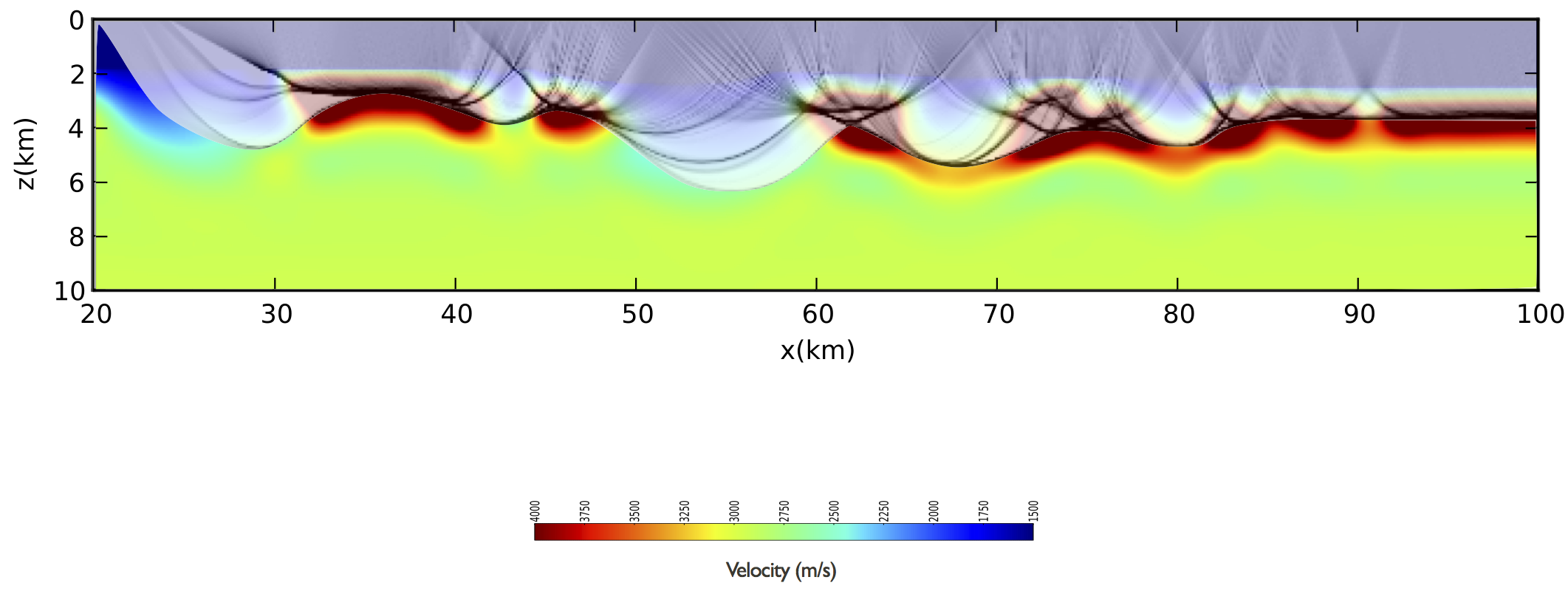
To get a reasonable starting model, we conducted first-break traveltime inversion on hand-picked traveltime from approximately 600k traces. We used the relatively noise-free high-frequency arrivals for this purpose. With these picks, we carried out a traveltime inversion, yielding a RMS traveltime misfit of only 11 ms. The result of this exercise, including the ray paths, is plotted in Figure initialgom. The lack of deep penetration of the rays clearly reveals the challenges we face for the recovery of the salt bodies. The hope of FWI is to improve the recovery of top and bottom salt and hence improve the quality of the sub-salt imaging. We want to accomplish this with minimal user intervention.
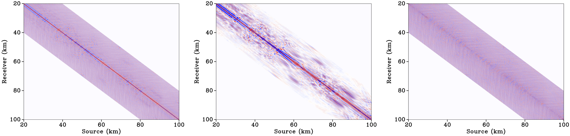
To overcome the extremely poor signal-to-noise at low frequencies, we carried out curvelet12-domain denoising on selected frequency slices (2-5 Hz) in the source-receiver domain. The denoising itself, consisted of solving a sparsity-promoting program to find the denoised curvelet-coefficients, followed by a debiasing step and the inverse curvelet transform, to recover the denoised frequency slices. An example of this sophisticated denoising procedure is included in Figure dnoise. This result clearly shows that we are able to remove a significant portion of the incoherent noise while preserving the amplitudes (there is very little coherent energy in the difference plot).
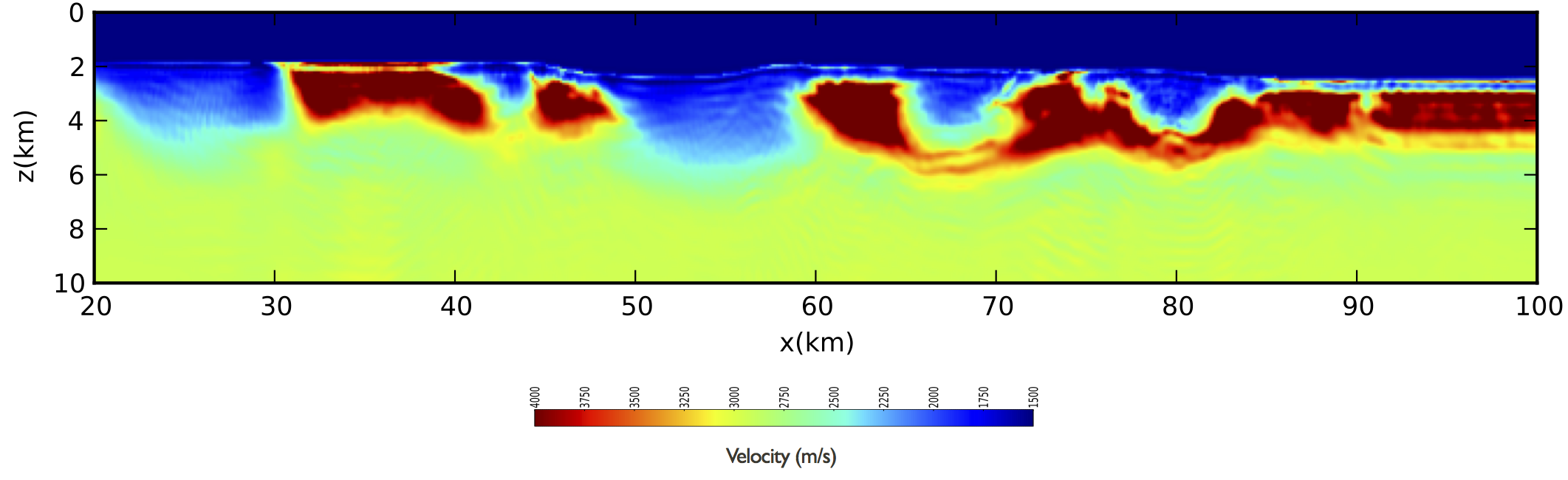
Given the denoised frequency slices, we ran our inversion in seven overlapping low-to-high frequency bands with four randomly selected frequencies per band. To help stabilize this multiscale inversion, we apply a nonlinear anisotropic smoothing by imposing a sparsity constraint on the curvelet-transform coefficients of the model updates, as described by Li et al. (2012). Since imposing this constraint calls for several iterations, we follow the frugal strategy of this paper by only working with 600 randomly selected shots out of a total of 3200 shots. The results of this exercise for six Gauss-Newton subproblems is included in Figure finalgom.
The output of this workflow is encouraging because we are evidently able to recover top salt with reasonable detail without the need of
reflection traveltime picking and salt floading that are part of the conventional velocity model building and migration workflows and which typically require large amounts of human intervention, and
data (pre)processing prior or during the inversion to remove the imprint of elastic phases in the data.
The latter feature is remarkable because we are able to get a reasonable inversion result for shallow depths without manipulating the data (except for the denoising of course). Because we are carrying out the inversion of the elastic data with an acoustic code, we had to limit the number of subproblems to prevent the algorithm from fitting the elastic phases. This also explains that we were only able to fit 21 percent of the data’s energy and that our result lacks details of the top salt.
While these results may be encouraging, there is still lots of room for improvement including
We presented a formulation of FWI that is cognizant of its often excessive and sometimes even unfeasible demand for computational resources by only calling for more data and accuracy of wave simulations as needed to guarantee convergence of the algorithm. This approach allowed us to conduct 3D FWI on a small machine. The same data reduction techniques enabled us to regularize FWI via nonlinear anisotropic curvelet-domain smoothing of the model updates. Application of this approach to the Chevron GOM dataset yielded reasonable results without extensive user intervention (except, of course, for the first-break picking to estimate the starting model). However, at depths exceeding 4km the starting model lacked information on the long-wavelength components of the salt. Because of the relatively short offset and missing low frequencies, FWI was unfortunately not able to recover these missing long-wavelength components of the salt.
Aside from the somewhat obvious calls for improvements resulting from our work on the GOM dataset, FWI more generally suffers fundamentally from lack of robustness with respect to outliers, e.g. unmodelled elastic phases in the data, and worse from local minima stemming from the highly nonlinear relationship between the medium properties and the data. Because “getting the physics right” really is an oxymoron, FWI requires a formulation that is less sensitive to noise, outliers in the data, and scaling by the source function. Early attempts towards such a formulation have appeared in the literature in recent work by Aravkin et al. (2012) on FWI with student’s t penalties and by Aravkin and van Leeuwen (2012) on the estimation of nuisance parameter with variable projection, which includes source estimation. As for the fundamental problem of mitigating the effects of local minima, several approaches have been proposed recently, including
a rigorous mathematical framework with frequency selection that guarantees convergence of steepest descents by a multi-level method that relaxes the parsimoniousness of the model as the frequency increases. This theoretical work by de Hoop, Qiu, and Scherzer (2012) has connections to the curvelet regularization we used to invert the GOM data. Unfortunately, this work merely guarantees convergence for certain starting models and does not remove the condition that the starting model needs to be accurate enough to fall in the region of convergence;
extension of FWI to include focussing. In this approach, advocated by Symes (2008) and Biondi and Almomin seeks to minimize the difference between the observed and simulated data while also minimizing a MVA-like objective. Aside from including the principle of focusing, this approach aims to remove local minima by increasing the degrees of freedom. While this leads to a computationally very challenging formulation (see van Leeuwen and Herrmann (2012) for a possible way around this computational problem ), there are indications that the larger degree of freedom partly eliminates the need of a highly accurate starting model, and
removal of the nonlinearity of FWI by working with an “all-at-once” approach (Ascher and Haber 2005) where the optimization is carried out over the wavefields as well as over the model parameters. Because of the increase of the degrees of freedom, we can also expect this approach to be less sensitive to local minima as was confirmed in recent work by Leeuwen and Herrmann (2013). This work proposes a new penalty method, which overcomes the infeasible storage demands of the all-at-once method.
This work was in part financially supported by the Natural Sciences and Engineering Research Council of Canada Discovery Grant (22R81254) and the Collaborative Research and Development Grant DNOISE II (375142-08). This research was carried out as part of the SINBAD II project with support from the following organizations: BG Group, BGP, BP, Chevron, ConocoPhillips, Petrobras, PGS, Total SA, and WesternGeco.
Aravkin, A. Y., and T. van Leeuwen. 2012. “Estimating nuisance parameters in inverse problems.” Inverse Problems 28 (11): 115016.
Aravkin, Aleksandr, Michael P. Friedlander, Felix J. Herrmann, and Tristan Leeuwen. 2012. “Robust inversion, dimensionality reduction, and randomized sampling.” Mathematical Programming 134 (1) (jun): 101–125. doi:10.1007/s10107-012-0571-6. http://www.springerlink.com/index/10.1007/s10107-012-0571-6.
Ascher, Uri M., and Eldad Haber. 2005. “Computational Methods for Large Distributed Parameter Estimation Problems in 3D.” In Modeling, Simulation and Optimization of Complex Processes, ed. HansGeorg Bock, HoangXuan Phu, Ekaterina Kostina, and Rolf Rannacher, 15–36. Springer Berlin Heidelberg. http://dx.doi.org/10.1007/3-540-27170-8\_2.
Biondi, Biondo, and Ali Almomin. “Tomographic full waveform inversion (TFWI) by combining full waveform inversion with wave-equation migration velocity anaylisis.” In SEG Technical Program Expanded Abstracts 2012, 1–5. doi:10.1190/segam2012-0275.1. http://library.seg.org/doi/abs/10.1190/segam2012-0275.1.
Friedlander, Michael P., and Mark Schmidt. 2012. “Hybrid Deterministic-Stochastic Methods for Data Fitting.” SIAM Journal on Scientific Computing 34 (3) (may): A1380–A1405. doi:10.1137/110830629. http://epubs.siam.org/doi/abs/10.1137/110830629.
Haber, Eldad, Matthias Chung, and Felix Herrmann. 2012. “An Effective Method for Parameter Estimation with PDE Constraints with Multiple Right-Hand Sides.” SIAM Journal on Optimization 22 (3) (jul): 739–757. doi:10.1137/11081126X. http://epubs.siam.org/doi/abs/10.1137/11081126X.
Hennenfent, G., and F. J. Herrmann. 2006. “Seismic denoising with non-uniformly sampled curvelets.” CISE 8 (3): 16–25.
de Hoop, Maarten V., Lingyun Qiu, and Otmar Scherzer. 2012. “A convergence analysis of a multi-level projected steepest descent iteration for nonlinear inverse problems in Banach spaces subject to stability constraints.” arXiv.org (jun).
Krebs, Jerome R., John E. Anderson, David Hinkley, Anatoly Baumstein, Sunwoong Lee, Ramesh Neelamani, and Martin-Daniel Lacasse. 2009. “Fast full wave seismic inversion using source encoding.” Geophysics 28 (1): 2273–2277. doi:10.1190/1.3255314. http://link.aip.org/link/SEGEAB/v28/i1/p2273/s1\&Agg=doi http://library.seg.org/vsearch/servlet/VerityServlet?KEY=SEGLIB\&smode=strresults\&sort=chron\&maxdisp=25\&threshold=0\&pjournals=SAGEEP,JEEGXX\&pjournals=JEEGXX\&pjournals=SAGEEP\&pjournals=GPYSA7,LEEDFF,SEGEAB,SEGBKS\&pjournals=GPYSA7\&pjournals=LEEDFF\&pjournals=SEGEAB\&pjournals=SEGBKS\&possible1zone=article\&possible4=krebs\&possible4zone=author\&bool4=and\&OUTLOG=NO\&viewabs=SEGEAB\&key=DISPLAY\&docID=5\&page=1\&chapter=0.
van Leeuwen, T., and Felix J. Herrmann. 2012. “Wave-equation extended images: computation and velocity continuation.” In EAGE technical program. EAGE. https://www.slim.eos.ubc.ca/Publications/Public/Conferences/EAGE/2012/vanleeuwen2012EAGEext/vanleeuwen2012EAGEext.pdf.
van Leeuwen, Tristan, Aleksandr Y. Aravkin, and Felix J. Herrmann. 2011. “Seismic waveform inversion by stochastic optimization.” International Journal of Geophysics 2011. https://www.slim.eos.ubc.ca/Publications/Public/Journals/InternationJournalOfGeophysics/2011/vanLeeuwen10IJGswi/vanLeeuwen10IJGswi.pdf.
Leeuwen, Tristan van, Dan Gordon, Rachel Gordon, and Felix J. Herrmann. 2012. “Preconditioning the Helmholtz equation via row-projections.” In EAGE technical program. EAGE. https://www.slim.eos.ubc.ca/Publications/Public/Conferences/EAGE/2012/vanleeuwen2012EAGEcarpcg/vanleeuwen2012EAGEcarpcg.pdf.
van Leeuwen, Tristan, and Felix J. Herrmann. 2012. “Fast waveform inversion without source-encoding.” Geophysical Prospecting (jul): no–no. doi:10.1111/j.1365-2478.2012.01096.x. http://doi.wiley.com/10.1111/j.1365-2478.2012.01096.x.
———. 2013. “3D frequency-domain seismic inversion using a row-projected helmholtz solver.” https://www.slim.eos.ubc.ca/Publications/Private/Submitted/2013/vanLeeuwen20133DFWI/vanLeeuwen20133DFWI.pdf.
Leeuwen, Tristan van, and Felix J. Herrmann. 2013. Mitigating local minima in full-waveform inversion by expanding the search space. https://www.slim.eos.ubc.ca/Publications/Private/Tech Report/2013/vanLeeuwen2013Penalty1/vanLeeuwen2013Penalty1.pdf.
Li, X., A. Y. Aravkin, T. van Leeuwen, and F. J. Herrmann. 2012. “Fast randomized full-waveform inversion with compressive sensing.” Geophysics 77 (3): A13. doi:10.1190/geo2011-0410.1.
Plessix, R.-E. 2006. “A review of the adjoint-state method for computing the gradient of a functional with geophysical applications.” Geophysical Journal International 167 (2): 495–503. http://dx.doi.org/10.1111/j.1365-246X.2006.02978.x.
Symes, W. W. 2008. “Migration Velocity Analysis and Waveform Inversion.” Geophysical Prospecting 56 (765-790).
Tarantola, A., and A. Valette. 1982. “Generalized nonlinear inverse problems solved using the least squares criterion.” Reviews of Geophysics and Space Physics 20 (2): 129–232.
Terentyev, I. S., T. Vdovina, W. W. Symes, X. Wang, and D. Sun. “IWAVE: a framework for wave simulation.”
Seismic Laboratory for Imaging and Modeling, Department of Earth, Ocean, and Atmospheric Sciences, the University of British Columbia, Canada.↩
Simon Frasier University, Canada.↩
Seismic Laboratory for Imaging and Modeling, Department of Earth, Ocean, and Atmospheric Sciences, the University of British Columbia, Canada.↩
Simon Frasier University, Canada.↩
Seismic Laboratory for Imaging and Modeling, Department of Earth, Ocean, and Atmospheric Sciences, the University of British Columbia, Canada.↩
Seismic Laboratory for Imaging and Modeling, Department of Earth, Ocean, and Atmospheric Sciences, the University of British Columbia, Canada.↩
Seismic Laboratory for Imaging and Modeling, Department of Earth, Ocean, and Atmospheric Sciences, the University of British Columbia, Canada.↩
Department of Earth, Ocean, and Atmospheric Sciences, the University of British Columbia, Canada.↩
University of Western Australia.↩
Seismic Laboratory for Imaging and Modeling, Department of Earth, Ocean, and Atmospheric Sciences, the University of British Columbia, Canada.↩
Or equivalently when we generate new supershots by aggregating sequential into simultaneous shots with amplitude or phase encoding (see e.g., (T. van Leeuwen and Herrmann 2012) and the references therein).↩
The 2D curvelet transform decomposes a two-dimensional function into localized plane waves that live in different frequency bands. Curvelets are sparse, i.e., there are only few large coefficients, because they only give rise to significant coefficients if the orientation and dominant bandwidth of the curvelet coincides with a localized event in the data. This makes this transform very suitable for denoising (see e.g., (Hennenfent and Herrmann 2006)).↩