![]()
![]()
Abstract
Adapting the cloud for high-performance computing (HPC) is a challenging task, as software for HPC applications hinges on fast network connections and is sensitive to hardware failures. Using cloud infrastructure to recreate conventional HPC clusters is therefore in many cases an infeasible solution for migrating HPC applications to the cloud. As an alternative to the generic lift and shift approach, we consider the specific application of seismic imaging and demonstrate a serverless and event-driven approach for running large-scale instances of this problem in the cloud. Instead of permanently running compute instances, our workflow is based on a serverless architecture with high throughput batch computing and event-driven computations, in which computational resources are only running as long as they are utilized. We demonstrate that this approach is very flexible and allows for resilient and nested levels of parallelization, including domain decomposition for solving the underlying partial differential equations. While the event-driven approach introduces some overhead as computational resources are repeatedly restarted, it inherently provides resilience to instance shut-downs and allows a significant reduction of cost by avoiding idle instances, thus making the cloud a viable alternative to on-premise clusters for large-scale seismic imaging.
Introduction
Seismic imaging of the earth’s subsurface is one of the most computationally expensive applications in scientific computing, as state-of-the-art imaging methods such as least-squares reverse time migration (LS-RTM), require repeatedly solving a large number of forward and adjoint wave equations during numerical optimization (e.g. Valenciano, 2008; Dong et al., 2012; P. A. Witte et al., 2019b). Similar to training neural networks, the gradient computations in seismic imaging are based on backpropagation and require storage or re-computations of the state variables (i.e. of the forward modeled wavefields). Due to the large computational cost of repeatedly modeling wave propagation over many time steps using finite difference modeling, seismic imaging requires access to high-performance computing (HPC) clusters, but the high cost of acquiring and maintaining HPC cluster makes this option only viable for a small number of major energy companies (“Seismic processing and imaging,” 2019). For this reason, cloud computing has lately emerged as a possible alternative to on-premise HPC clusters, offering many advantages such as no upfront costs, a pay-as-you-go pricing model and theoretically unlimited scalability. Outside of the HPC community, cloud computing is today widely used by many companies for general purpose computing, data storage and analysis or machine learning. Customers of cloud providers include major companies such as General Electric (GE), Comcast, Shell or Netflix, with the latter hosting their video streaming content on Amazon Web Services (AWS) (“AWS enterprise customer success stories,” 2019).
However, adapting the cloud for high-performance computing applications such as seismic imaging, is not straight-forward, as numerous investigations and case studies have shown that performance, latency, bandwidth and mean time between failures (MTBF) in the cloud can vary significantly between platform providers, services and hardware, and are often inferior compared to on-premise HPC resources. Especially in the early days of cloud computing, performance and network connections were considerably slower than on comparable on-premise HPC systems, as discussed in a number of publications. An early performance analysis by Jackson et al. (2010) of a range of typical NERSC HPC applications on Amazon’s Elastic Compute Cloud (EC2) found that, at the time of the comparison in 2010, applications on EC2 ran several orders of magnitude slower than on comparable HPC systems, due to low bandwidth and high latency. Other performance benchmarks from the late 2000s and early 2010s, similarly conclude that poor network performance severely limited the HPC capabilities of the cloud at that time (Garfinkel, 2007; Napper and Bientinesi, 2009; Iosup et al., 2011; Jackson et al., 2011; Ramakrishnan et al., 2012; Mehrotra et al., 2016). Cloud providers have since then responded by making significant improvements regarding network connections, now offering technologies such as InfiniBand, specialized network adapters such as Amazon’s elastic fabric adapter (EFA, “AWS elastic fabric adapter,” 2019) and improved virtualization techniques to improve performance (e.g. AWS Nitro, “AWS Nitro system,” 2019). Accordingly, more recent benchmarks on various cloud platforms, including AWS and Microsoft Azure, find that the performance on newly introduced HPC instances is oftentimes on par with modern on-premise HPC systems (Scheuner and Leitner, 2018; Kotas et al., 2018). Nevertheless, enhanced network technologies are typically limited to a small subset of specialized HPC instances, which are not as widely available as general purpose instances and which are accordingly more expensive (“AWS documentation,” 2019a).
Aside from network communication, several investigations (Gupta and Milojicic, 2011; Sadooghi et al., 2017; Kotas et al., 2018) point out that embarrassingly parallel applications show very good performance that is comparable to (non-virtualized) HPC environments, even in the early days of the cloud and using standard (non-HPC optimized) nodes. Similarly, performance tests on single cloud nodes and bare-metal instances using HPCC and high-performance LINPACK benchmarks demonstrate good performance and scalability as well (Rad et al., 2015; Mohammadi and Bazhirov, 2018). These findings underline that the lift and shift approach for porting HPC applications to the cloud is unfavorable, as most HPC codes are based on highly synchronized message passing (i.e. MPI, W. Gropp et al., 1999) and rely on stable and fast network connections, which are only available on certain (limited) instance types and which are thus more expensive. On the other hand, individual compute nodes and architectures offered by cloud computing are indeed comparable to current supercomputing systems (Mohammadi and Bazhirov, 2018) and the cloud offers a range of novel technologies such as cloud object storage or event-driven computations (“AWS documentation,” 2019h). These technologies are not available on traditional HPC systems and make it possible to address computational bottlenecks of HPC in fundamentally new ways. Porting HPC applications to the cloud in a way that is financially viable therefore requires a careful re-architecture of the corresponding codes and software stacks to take advantage of these technologies, while minimizing communication and idle times. This process is heavily application dependent and requires the identification of how specific applications can take advantage of specialized cloud services such as serverless compute or high throughput batch processing to mitigate resilience issues and minimize cost, while avoiding idle instances and fast network fabrics where possible.
Based on these premises, we present a workflow for large-scale seismic imaging on AWS, which does not rely on a conventional cluster of virtual machines, but is instead based on a serverless workflow that takes advantage of the mathematical properties of the seismic imaging optimization problem (Friedman and Pizarro, 2017). Similar to deep learning, objective functions in seismic imaging consist of a sum of (convex) misfit functions and iterations of associated optimization algorithms exhibit the structure of a MapReduce program (Dean and Ghemawat, 2008). The map part corresponds to computing the gradient of each element in the sum and is embarrassingly parallel to compute, but individual gradient computations are expensive as they involve solving partial differential equations (PDEs). The reduce part corresponds to the summation of the gradients and update of the model parameters and is comparatively cheap to compute, but I/O intensive. Instead of performing these steps on a cluster of permanently running compute instances, our workflow is based on specialized AWS services such as AWS Batch and Lambda, which are responsible for automatically launching and terminating the required computational resources (“AWS documentation,” 2019g, 2019h). EC2 instances are only running as long as they are utilized and are shut down automatically as soon as computations are finished, thus preventing instances from sitting idle. This stands in contrast to alternative MapReduce cloud services, such as Amazon’s Elastic Map Reduce (EMR), which is based on Apache Hadoop and relies on a cluster of permanently running EC2 instances (“AWS documentation,” 2019c). In our approach, expensive gradient computations are carried out by AWS Batch, a service for processing embarrassingly parallel workloads, but with the possibility of using (MPI-based) domain decomposition for individual solutions of partial differential equations (PDEs). The cheaper gradient summations are performed by Lambda functions, a service for serverless computations, in which code is run in response to events, without the need to manually provision computational resources (“AWS documentation,” 2019h).
The following section provides an overview of the mathematical problem that underlies seismic imaging and we identify possible characteristics that can be taken advantage of to avoid the aforementioned shortcomings of the cloud. In the subsequent section, we describe our seismic imaging workflow, which has been developed specifically for AWS, but the underlying services are available on other cloud platforms (Google Compute Cloud, Azure) as well. We then present a performance analysis of our workflow on a real-world seismic imaging application, using a popular subsurface benchmark model (Billette and Brandsberg-Dahl, 2005). Apart from conventional scaling tests, we also consider specific cloud metrics such as resilience and cost, which, aside from the pure performance aspects like scaling and time-to-solution, are important practical considerations for HPC in the cloud. An early application of our workflow is presented in an expanded conference abstract (P. A. Witte et al., 2019d).
Problem overview
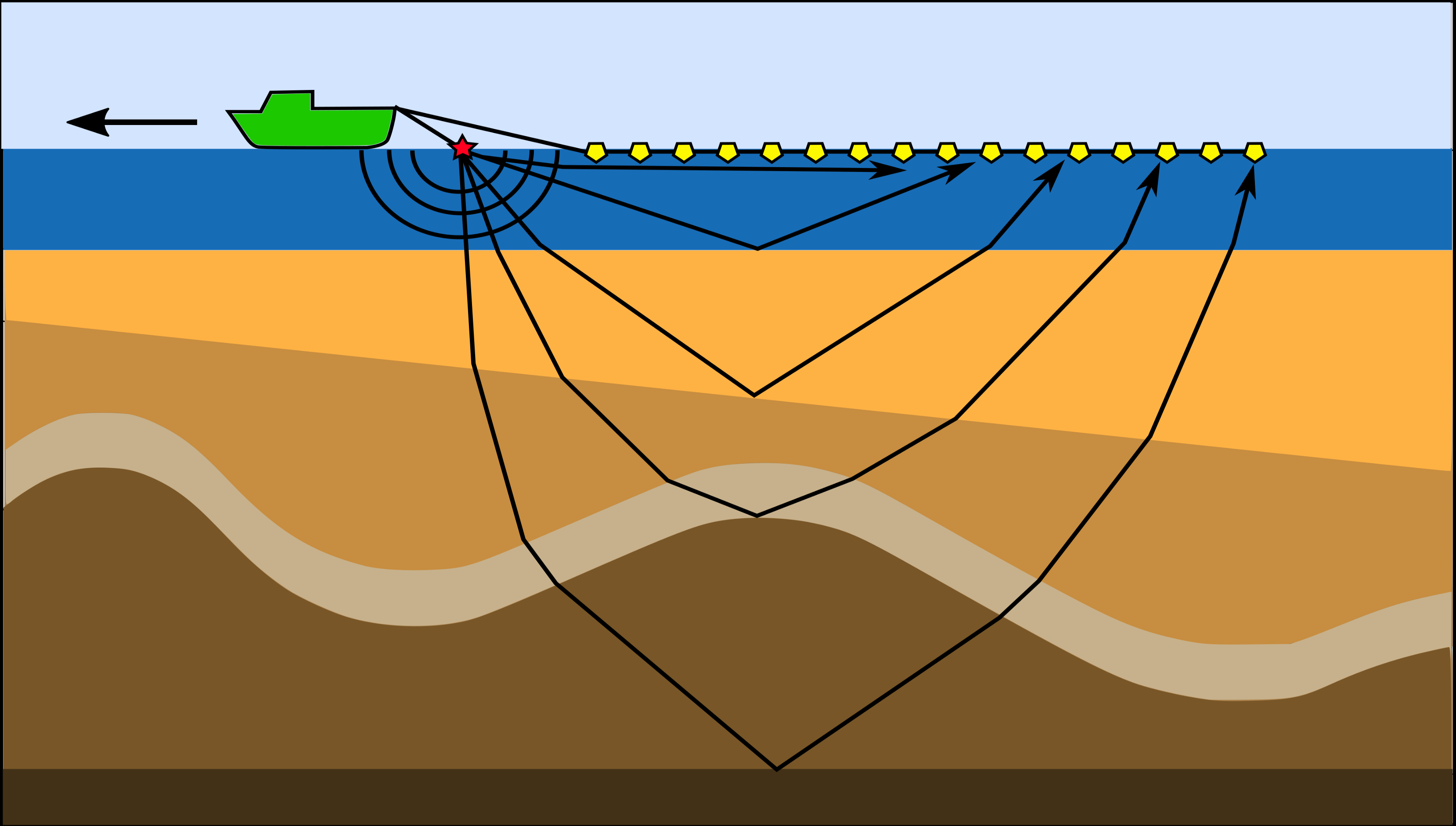
Seismic imaging and parameter estimation are a set of computationally challenging inverse problems with high practical importance, as they are today widely used for geophysical exploration and monitoring geohazards. Exploration seismology is based on the manual excitation of seismic sources, which trigger sound and/or elastic waves that travel through the subsurface. At geological interfaces, waves are scattered and reflected, causing parts of the wavefield to travel back to the surface, where it is recorded by an array of receivers (Figure 1). In a seismic survey, the source is fired repeatedly as it moves across the survey area and the observed data that is collected for each source location is denoted by \(\mathbf{d}_i\). The objective of seismic imaging is to recover a physical parametrization of the subsurface from the recorded seismic data. In the setting of inverse problems, this is achieved by minimizing the misfit between recorded data and data that is predicted using numerical modeling. The forward problem is defined as the computation of a predicted seismic shot record through a forward modeling operator \(\mathcal{F}(\mathbf{m}, \mathbf{q}_i)\), where \(\mathbf{m}\) denotes the discretized unknown parameters, such as the seismic image or the acoustic wave speed and the vector \(\mathbf{q}_i\) represents the location and the time signature of the seismic source. The evaluation of the forward modeling operator corresponds to numerically solving a discretized version of the wave equation for the given set of model parameters and current source location using for example finite differences (details are given in Appendix A).
In the inverse problem, we are interested in recovering the parameters \(\mathbf{m}\) from the observed seismic data \(\mathbf{d}_i\). Mathematically, this is achieved by formulating an unconstrained optimization problem in which we minimize the \(\ell_2\)-misfit between the observed and numerically modeled data (Tarantola, 1984; Virieux and Operto, 2009): \[ \begin{equation} \underset{\mathbf{m}}{\operatorname{minimize}} \hspace{0.2cm} \Phi(\mathbf{m}) = \sum_{i=1}^{n_s} \frac{1}{2}||\mathcal{F}(\mathbf{m}, \mathbf{q}_i) - \mathbf{d}_i ||^2_2. \label{eq1} \end{equation} \] In essence, the goal of seismic inversion is to find a set of model parameters \(\mathbf{m}\), such that the numerically modeled data matches the observed data from the seismic survey. The total number of individual source experiments \(n_s\) for realistic surveys, i.e. the number of PDEs that have to solved for each evaluation of \(\Phi(\mathbf{m})\), is quite large and lies in the range of \(10^3\) for 2D surveys and \(10^5\) for 3D surveys.
Seismic inverse problems of this form are typically solved with gradient-based optimization algorithms such as (stochastic) gradient descent, (Gauss-) Newton methods, sparsity-promoting minimization or constrained optimization (e.g. Pratt, 1999; Peters et al., 2019) and therefore involve computing the gradient of Equation \(\ref{eq1}\) for all or a subset of indices \(i\). The gradient of the objective function is given by: \[ \begin{equation} \mathbf{g} = \sum_{i=1}^{n_s} \mathbf{J}^\top \Big( \mathcal{F}(\mathbf{m}, \mathbf{q}_i) - \mathbf{d}_i \Big), \label{eq2} \end{equation} \] where the linear operator \(\mathbf{J} = \frac{\partial \mathcal{F}(\mathbf{m}, \mathbf{q}_i)}{\partial \mathbf{m}}\) is the partial derivative of the forward modeling operator with respect to the model parameters \(\mathbf{m}\) and \(\top\) denotes the matrix transpose. Both the objective function, as well as the gradient exhibit a sum structure over the source indices and are embarrassingly parallel to compute. Evaluating the objective function and computing the gradient are therefore instances of a MapReduce program (Dean and Ghemawat, 2008), as they involve the parallel computation and subsequent summation of elements of the sum. However, computing the gradient for a single index \(i\) involves solving two PDEs, namely a forward wave equation and an adjoint (linearized) wave equation (denoted as a multiplication with \(\mathbf{J}^\top\)). For realistically sized 3D problems, the discretized model in which wave propagation is modeled has up to \(10^9\) variables and modeling has to be performed for several thousand time steps. The observed seismic data \(\mathbf{d}_i\) (\(i=1,...,n_s\)) is typically in the range of several terabytes and a single element of the data (a seismic shot record) ranges from several mega- to gigabytes.
The problem structure of equation \(\ref{eq1}\) is very similar to deep learning and the parallels between convolutional neural networks and PDEs have lately attracted strong attention (Lars Ruthotto and Haber, 2018). As in deep learning, computing the gradient of the objective function (equation \(\ref{eq2}\)) is based on backpropagation and in principle requires storing the state variables of the forward problem. However, in any realistic setting the wavefields are too big to be stored in memory and therefore need to be written to secondary storage devices or recomputed from a subset of checkpoints (Griewank and Walther, 2000). Alternatively, domain decomposition can be used to reduce the domain size per compute node such that the forward wavefields fit in memory, or time-to frequency conversion methods can be employed to compute gradients in the frequency domain (Furse, 1998; P. A. Witte et al., 2019b). In either case, computing the gradient for a given index \(i\) is expensive both in terms of necessary floating point operations, memory and IO and requires highly optimized finite-difference modeling codes for solving the underlying wave equations. Typical computation times of a single (3D-domain) gradient \(\mathbf{g}_i\) (i.e. one element of the sum) are in the range of minutes to hours, depending on the domain size and the complexity of the wave simulator, and the computations have to be carried out for a large number of source locations and iterations.
The high computational cost of seismic modeling, in combination with the complexity of implementing optimization algorithms to solve equation \(\ref{eq1}\), leads to enormously complex inversion codes, which have to run efficiently on large-scale HPC clusters. A large amount of effort goes into implementing fast and scalable wave equation solvers (Abdelkhalek et al., 2009; M. Louboutin et al., 2019), as well as into frameworks for solving the associated inverse problem (Symes et al., 2011; L. Ruthotto et al., 2017; Silva and Herrmann, 2017; P. A. Witte et al., 2019c). Codes for seismic inversion are typically based on message passing and use MPI to parallelize the loop of the source indices (equation \(\ref{eq1}\)). Furthermore, a nested parallelization is oftentimes used to apply domain-decomposition or multi-threading to individual PDE solves. The reliance of seismic inversion codes on MPI to implement an embarrassingly parallel loop is disadvantageous in the cloud, where the mean-time-between failures (MTBF) is much shorter than on HPC systems (Jackson et al., 2010) and instances using spot pricing can be arbitrarily shut down at any given time (“AWS documentation,” 2019j). Another important aspect is that the computation time of individual gradients can vary significantly and cause load imbalances, which is problematic in the cloud, where users are billed for running instances by the second, regardless of whether the instances are in use or idle. For these reasons, we present an alternative approach for seismic imaging in the cloud based on batch processing and event-driven computations.
Event-driven seismic imaging on AWS
Workflow
Optimization algorithms for minimizing equation \(\ref{eq1}\) essentially consists of three steps. First, the elements of the gradient \(\mathbf{g}_i\) are computed in parallel for all or a subset of indices \(i \in n_s\), which corresponds to the map part of a MapReduce program. The number of indices for which the objective is evaluated defines the batch size of the gradient. The subsequent reduce part consists of summing these elements into a single array and using them to update the unknown model/image according to the rule of the respective optimization algorithm (Algorithm 1). Optimization algorithms that fit into this general framework include variations of stochastic/full gradient descent (GD), such as Nesterov’s accelerated GD (Nesterov, 2018) or Adam (Kingma and Ba, 2014), as well as the nonlinear conjugate gradient method (Fletcher and Reeves, 1964), projected GD or iterative soft thresholding (Beck and Teboulle, 2009). Conventionally, these algorithms are implemented as a single program and the gradient computations for seismic imaging are parallelized using message passing. Running MPI-based programs of this structure in the cloud require that users request a set of EC2 instances and establish a network connection between all workers (“AWS documentation,” 2019b). Tools like StarCluster (“StarCluster,” 2019) or AWS HPC (“AWS High Performance Computing,” 2019) facilitate the process of setting up a cluster and even allow adding or removing instances to a running cluster. However, adding or dropping instances/nodes during the execution of an MPI program is not easily possible, so the number of instances has to stay constant during the entire length of the program execution, which, in the case of seismic inversion, can range from several days to weeks. This makes this approach not only prone to resilience issues, but it can result in significant cost overhead, if workloads are unevenly distributed and instances are temporarily idle.
1. Input: batch size \(n_b\), max. number of iterations \(n\), step size \(\alpha\), initial guess \(\mathbf{m}_1\)
2. for \(k=1,...,n\)
3. Compute gradients \(\mathbf{g}_i\), \(i=1, ..., n_b\) in parallel
4. Sum gradients: \(\mathbf{g} = \sum_{i=1}^{n_b} \mathbf{g}_i\)
5. Update optimization variable, e.g. using GD: \(\mathbf{m}_{k+1} = \mathbf{m}_{k} - \alpha \mathbf{g}\)
6. end
Instead of implementing and running optimization algorithms for seismic inverse problems as a single program that runs on a cluster of EC2 instances, we express the steps of a generic optimization algorithm through AWS Step Functions (Figure 2) and deploy its individual components through a range of specialized AWS services (“AWS documentation,” 2019i). Step functions allow the description of an algorithm as a collection of states and their relationship to each other using the JavaScript Object Notation (JSON). From the JSON definition of a workflow, AWS renders an interactive visual workflow in the web browser, as shown in Figure 2. For our purpose, we use Step Functions to implement our iterative loop (“Iterating a loop using Lambda,” 2018), during which we compute and sum the gradients, and use them to update the seismic image. We choose Step Functions to express our algorithm, as they allow composing different AWS Services such as AWS Batch and Lambda functions into a single workflow, thus making it possible to leverage preexisiting AWS services and to combine them into a single application. Another important aspect of Step Functions is that the execution of the workflow itself is managed by AWS and does not require running any EC2 instances, which is why we refer to this approach as serverless. During execution time, AWS automatically progresses the workflow from one state to the next and users are only billed for transitions between states, but the cost is negligible compared to the cost of running EC2 instances (0.025$ per 1,000 state transitions).
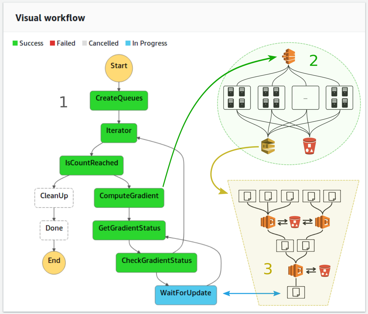
WaitForUpdate state, the workflow automatically progresses to the next iteration.States can be simple if-statements such as the IsCountReached state, which keeps track of the iteration number and terminates the workflow after a specified number of iterations, but states can also be used invoke other AWS services. Specifically, states can be used to invoke AWS Lambda functions to carry out serverless computations. Lambda functions allow users to run code in response to events, such as invocations through AWS Step Functions, and automatically assign the required amount of computational resources to run the code. Billing is based on the execution time of the code and the amount of used memory. Compared to EC2 instances, Lambda functions have a much shorter startup time in the range of milliseconds rather than minutes, but they are limited to 3 GB of memory and an execution time of 15 minutes. As such, Lambda functions themselves are not suitable for carrying out the gradient computations, but they can be used to manage other AWS services. In our workflow, we use Lambda functions invoked by the ComputeGradient state (Figure 2) to launch AWS Batch jobs for computing the gradients. During the gradient computation, which can take up to several hours, the Step Functions check in a user-defined interval if the full gradient has been computed, before advancing the workflow to the next state. The WaitForUpdate state pauses the workflow for a specified amount of time, during which no additional computational resources are running other than the AWS Batch job itself.
Computing the gradient
The gradient computations (equation 2) are the major workload of seismic inversion, as they involve solving forward and adjoint wave equations, but the embarrassingly parallel structure of the problem lends itself to high-throughput batch computing. On AWS, embarrassingly parallel workloads can be processed with AWS Batch, a service for scheduling and running parallel containerized workloads on EC2 instances (“AWS documentation,” 2019g). Parallel workloads, such as computing a gradient of a given batch size, are submitted to a batch queue and AWS Batch automatically launches the required EC2 instances to process the workload from the queue. Each job from the queue runs on an individual instance or set of instances, with no communication being possible between individual jobs.
In our workflow, we use the Lambda function invoked by the ComputeGradient state (Figure 2) to submit the gradient computations to an AWS Batch queue. Each element of the gradient \(\mathbf{g}_i\) corresponds to an individual job in the queue and is run by AWS Batch as a separate Docker container (“Docker,” 2019). Every container computes the gradient for its respective source index \(i\) and writes its resulting gradient to an S3 bucket (Figure 3), Amazon’s cloud object storage system (“AWS documentation,” 2019e). The gradients computed by our workflow are one-dimensional numpy arrays of the size of the vectorized seismic image and are stored in S3 as so-called objects (Van Der Walt et al., 2011). Once an individual gradient \(\mathbf{g}_i\) has been computed, the underlying EC2 instance is shut down automatically by AWS Batch, thus preventing EC2 instances from idling. Since no communication between jobs is possible, the summation of the individual gradients is implemented separately using AWS Lambda functions. For this purpose, each jobs also sends its S3 object identifier to a message queue (SQS) (“AWS documentation,” 2019d), which automatically invokes the reduction stage (Figure 4). For the gradient computations, each worker has to download the observed seismic data of its respective source index from S3 and the resulting gradient has to be uploaded to S3 as well. The bandwidth with which objects are up- and downloaded is only limited by the network bandwidth of the EC2 instances and ranges from 10 to 100 Gbps (“AWS documentation,” 2019a). Notably, cloud object storage such as S3 has no limit regarding the number of workers that can simultaneously read and write objects, as data is (redundantly) distributed among physically separated data centers, thus providing essentially unlimited IO scalability (“AWS documentation,” 2019e).

AWS Batch runs jobs from its queue as separate containers on a set of EC2 instances, so the source code of the application has to be prepared as a Docker container. Containerization facilitates portability and has the advantage that users have full control over managing dependencies and packages. Our Docker image contains the code for solving acoustic wave equations to compute gradients of a respective seismic source location. Since this is the most computational intensive part of our workflow, it is important that the wave equation solver is optimized for performance, but is also implemented in a programming language that allows interfacing other AWS services such as S3 or SQS. In our workflow, we use a domain-specific language compiler called Devito for implementing and solving the underlying wave equations using time-domain finite-difference modeling (M. Louboutin et al., 2019; Luporini et al., 2018). Devito is implemented in Python and provides an application programming interface (API) for implementing forward and adjoint wave equations as high-level symbolic expressions based on the SymPy package (Joyner et al., 2012). During runtime, the Devito compiler applies a series of performance optimizations to the symbolic operators, such as reductions of the operation count, loop transformations, and introduction of parallelism (Luporini et al., 2018). Devito then generates optimized finite-difference stencil code in C from the symbolic Python expressions and dynamically compiles and runs it. Devito supports both multi-threading using OpenMP, as well as generating code for MPI-based domain decomposition. Its high-level API allows expressing wave equations of arbitrary stencil orders or various physical representations without having to implement and optimize low-level stencil codes by hand. The complexity of implementing highly optimized and parallel wave equation solvers is therefore abstracted and vertically integrated into the AWS workflow.
By default, AWS Batch runs the container of each job on a single EC2 instance, but recently AWS introduced the possibility to run multi-node batch computing jobs (Rad et al., 2018). Thus, individual jobs from the queue can be computed on a cluster of EC2 instances and the corresponding Docker containers can communicate via the AWS network. In the context of seismic imaging and inversion, multi-node batch jobs enable nested levels of parallelization, as we can use AWS Batch to parallelize the sum of the source indices, while using MPI-based domain decomposition and/or multi-threading for solving the underlying wave equations. This provides a large amount of flexibility in regard of the computational strategy for performing backpropagation and how to address the storage of the state variables. AWS Batch allows to scale horizontally, by increasing the number of EC2 instances of multi-node jobs, but also enables vertical scaling by adding additional cores and/or memory to single instances. In our performance analysis, we compare and evaluate different strategies for computing gradients with Devito regarding scaling, costs and turnaround time.
Gradient reduction
Every computed gradient is written by its respective container to an S3 bucket, as no communication between individual jobs is possible. Even if all gradients in the job queue are computed by AWS Batch in parallel at the same time, we found that the computation time of individual gradients typically varies considerably (up to 10 percent), due to varying network performance or instance capacity. Furthermore, we found that the startup time of the underlying EC2 instances itself is highly variable as well, so jobs in the queue are usually not all started at the same time. Gradients therefore arrive in the bucket over a large time interval during the batch job. For the gradient reduction step, i.e. the summation of all gradients into a single array, we take advantage of the varying time-to-solutions by implementing an event-driven gradient summation using Lambda functions. In this approach, the gradient summation is not performed by as single worker or the master process who has to wait until all gradients have been computed, but instead summations are carried out by Lambda functions in response to gradients being written to S3.
The event-driven gradient summation is automatically invoked through SQS messages, which are sent by the AWS Batch workers that have completed their computations and have saved their respective gradient to S3. Before being shut down, every batch worker sends a message with the corresponding S3 object name to an AWS SQS queue, in which all object names are collected (Figure 4). Sending messages to SQS invokes AWS Lambda functions that read up to 10 messages at a time from the queue. Every invoked Lambda function that contains at least two messages, i.e. two object names, reads the corresponding arrays from S3, sums them into a single array, and writes the array as a new object back to S3. The new object name is sent to the SQS queue, while the previous objects and objects names are removed from the queue and S3. The process is repeated recursively until all \(n_b\) gradients have been summed into a single array, with \(n_b\) being the batch size for which the gradient is computed.
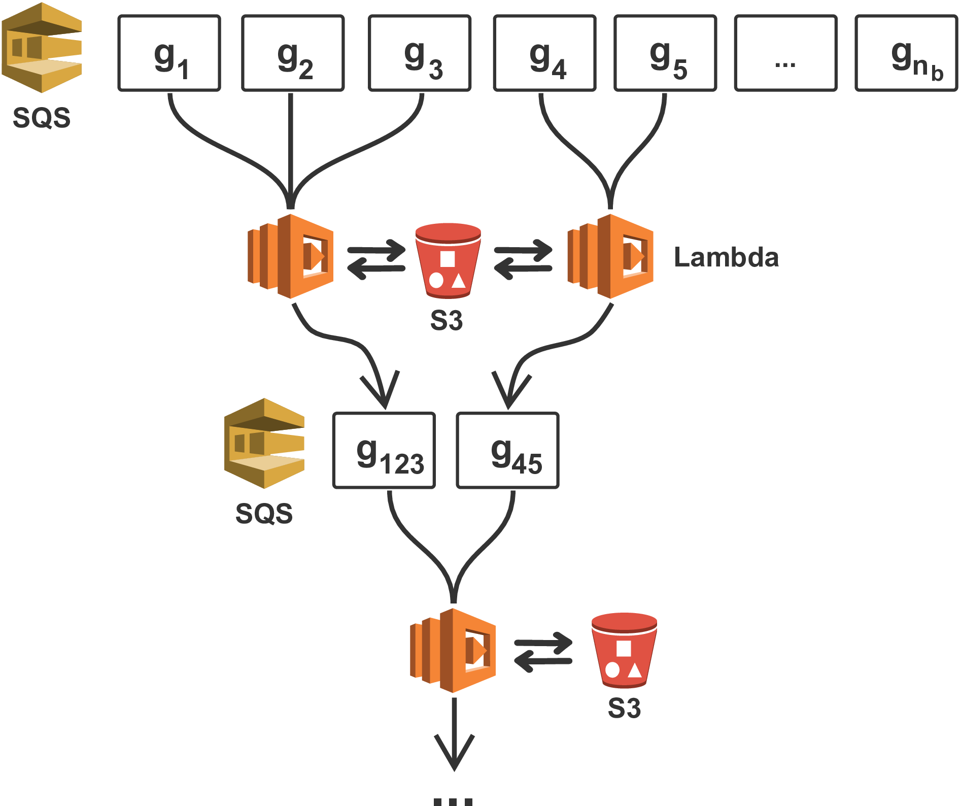
Since Lambda functions are limited to 3 GB of memory, it is not always possible to read the full gradient objects from S3. Gradients that exceed Lambda’s available memory are therefore streamed from S3 using appropriate buffer sizes and are re-uploaded to S3 using the multipart\_upload functions of the S3 Python interface (“Boto 3 documentation,” 2019). As the execution time of Lambda functions is furthermore limited to 15 minutes, the bandwidth of S3 is not sufficient to stream and re-upload objects that exceed a certain size within a single Lambda invocation. For this case, we include the possibility that the workers of the AWS Batch job split the computed gradients into smaller chunks that are saved separately in S3, with the respective objects names being sent to multiple SQS queues. The gradient summation is then performed in chunks by separate queues and Lambda functions. The CreateQueues task of our Step Functions workflow (Figure 2) automatically creates the required number of queues before starting the optimization loop and the CleanUp state removes them after the final iteration.
The advantage of the event-based gradient reduction is that that the summation is executed asynchronously, as soon as at least two S3 objects are available, while other batch jobs are still running. Therefore, by the time the last batch worker finishes the computation of its respective gradient, all remaining gradients have already been summed into a single object, or at least a small number of objects. Furthermore, summing files of a single queue happens in parallel (if enough messages are in the queue), as multiple Lambda functions can be invoked at the same time. Furthermore, splitting the gradients itself into chunks that are processed by separate queues leads to an additional layer of parallelism. In comparison to a fixed cluster of EC2 instances, the event-driven gradient summation using Lambda function also takes advantage of the fact that the summation of arrays is computationally considerably cheaper than solving wave equations and therefore does not require to be carried out on the expensive EC2 instances used for the PDE solves.
Variable update
Once the gradients have been computed and summed into a single array that is stored as an S3 object, the gradient is used to update the optimization variables of equation 1, i.e. the seismic image or subsurface parameters such as velocity. Depending on the specific objective function and optimization algorithm, this can range from simple operations like multiplications with a scalars (gradient descent) to more computational expensive operations such as sparsity promotion or applying constraints (Nocedal and Wright, 2006). Updates that use entry-wise operations only and are cheap to compute such as multiplications with scalars or soft-thresholding, can be applied directly by Lambda functions in the final step of the gradient summation. I.e. the Lambda function that sums the final two gradients, also streams the optimization variable of the current iteration from S3, uses the gradient to update it and directly writes the updated variable back to S3.
Many algorithms require access to the full optimization variable and gradient, such as Quasi-Newton methods and other algorithms that need to compute gradient norms. In this case, the variable update is too expensive and memory intensive to be carried out by Lambda functions and has to be submitted to AWS Batch as a single job, which is then executed on a larger EC2 instance. This can be accomplished by adding an extra state such as UpdateVariable to our Step Functions workflow. However, to keep matters simple, we only consider a simple stochastic gradient descent example with a fixed step size in our performance analysis, which is computed by the Lambda functions after summing the final two gradients (Bottou, 2010). The CheckUpdateStatus state of our AWS Step Functions advances the workflow to the next iteration, once the updated image (or summed gradient) has been written to S3. The workflow shown in Figure 2 terminates the optimization loop after a predefined number of iterations (i.e. epochs), but other termination criteria based on gradient norms or function values are possible too. The update of the optimization variable concludes a single iteration of our workflow, whose performance we will now analyze in the subsequent sections.
Performance analysis
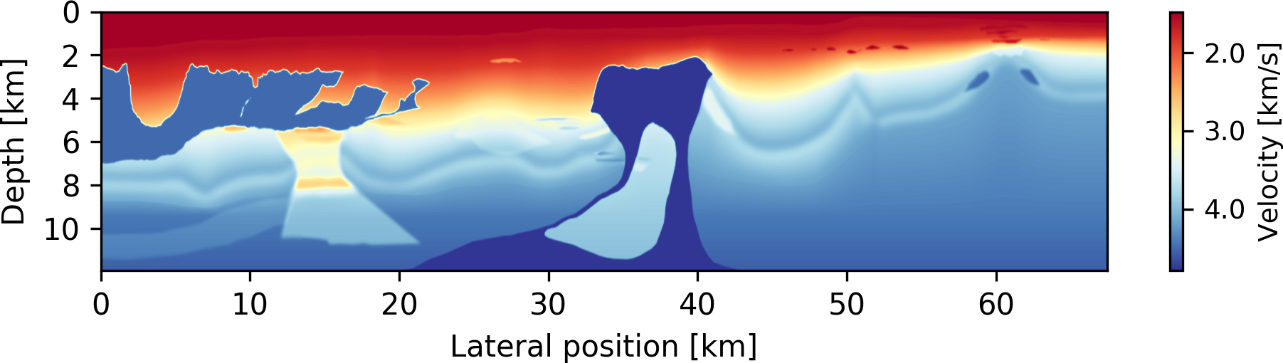
In our performance analysis, we are interested in the performance of our workflow on a real-world seismic imaging application regarding scalability, cost and turn-around time, as well as the computational benefits and overhead introduced by our event-driven approach. We conduct our analysis on a popular 2D subsurface velocity model (Figure 4), called the 2004 BP velocity estimation benchmark model (Billette and Brandsberg-Dahl, 2005). This model was originally created for analyzing seismic processing or inversion algorithms, but as the model represents a typical large-scale 2D workload, we consider this model for our following performance analysis. The seismic data set of this model contains \(1,348\) seismic source locations and corresponding observations \(\mathbf{d}_i\) (\(i=1, ..., 1,348\)). The (unknown) seismic image has dimensions of \(1,911 \times 10,789\) grid points, i.e. a total of almost 21 million parameters.

Weak scaling
In our first performance test, we analyze the weak scaling behavior of our workflow by varying the batch size (i.e. the number of source locations) for which the gradient of the LS-RTM objective function (Equation \(\ref{eq1}\)) is computed. For this test, we perform a single iteration of stochastic gradient descent (SGD) using our workflow and measure the time-to-solution as a function of the batch size. The workload per instance, i.e. per parallel worker, is fixed to one gradient. The total workload for a specified batch size is submitted to AWS Batch as a so-called array job, where each array entry corresponds to a single gradient \(\mathbf{g}_i\). AWS Batch launches one EC2 instance per array entry (i.e. per gradient), runs the respective container on the instance and then terminates the instance.
In the experiment, we measure the time-to-solution for performing a single iteration of our workflow, i.e. one stochastic gradient descent update. Therefore, each run involves the following steps:
A Lambda function submits the AWS Batch job for specified batch size \(n_b\) (Figure 3)
Compute gradients \(\mathbf{g}_i\) (\(i=1,...,n_b\)) in parallel (Figure 3)
Lambda functions sum the gradients (Figure 4): \(\mathbf{g} = \sum_{i=1}^{n_b} \mathbf{g}_i\)
A Lambda function performs the SGD update of the image: \(\mathbf{x} = \mathbf{x} - \alpha \mathbf{g}\)
We define the time-to-solution as the the time interval between the submission of the AWS Batch job by a Lambda function (step 1) and the time stamp of the S3 object containing the updated image (step 4). This time interval represents a complete iteration of our workflow.
The computations of the gradients are performed on m4.4xlarge instances (Appendix B) and the number of threads per instance is fixed to 8, which is the number of physical cores that is available on the instance. The m4 instance is a general purpose EC2 instance and we chose the instance size (4xlarge) such that we are able to store the wavefields for backpropagation in memory. The workload for each batch worker consists of solving a forward wave equation to model the predicted seismic data and an adjoint wave equation to backpropagate the data residual and to compute the gradient. For this and all remaining experiments, we use the acoustic isotropic wave equation with a second order finite difference (FD) discretization in time and 8th order in space. We model wave propagation for 12 seconds, which is the recording length of the seismic data. The time stepping interval is given by the Courant-Friedrichs-Lewy condition with 0.55 ms, resulting in 21,889 time steps. Since it is not possible for the waves to propagate through the whole domain within this time interval, we restrict the modeling grid to a size of \(1,911 \times 4,001\) grid points around the current source location. After modeling, each gradient is extended back to the full model size (\(1,911 \times 10,789\) grid points). The dimensions of this example represent a large-scale 2D example, but all components of our workflow are agnostic to the number of physical dimensions and are implemented for three-dimensional domains as well. The decision to limit the examples to a 2D model was purely made from a financial viewpoint and to make the results reproducible in a reasonable amount of time.
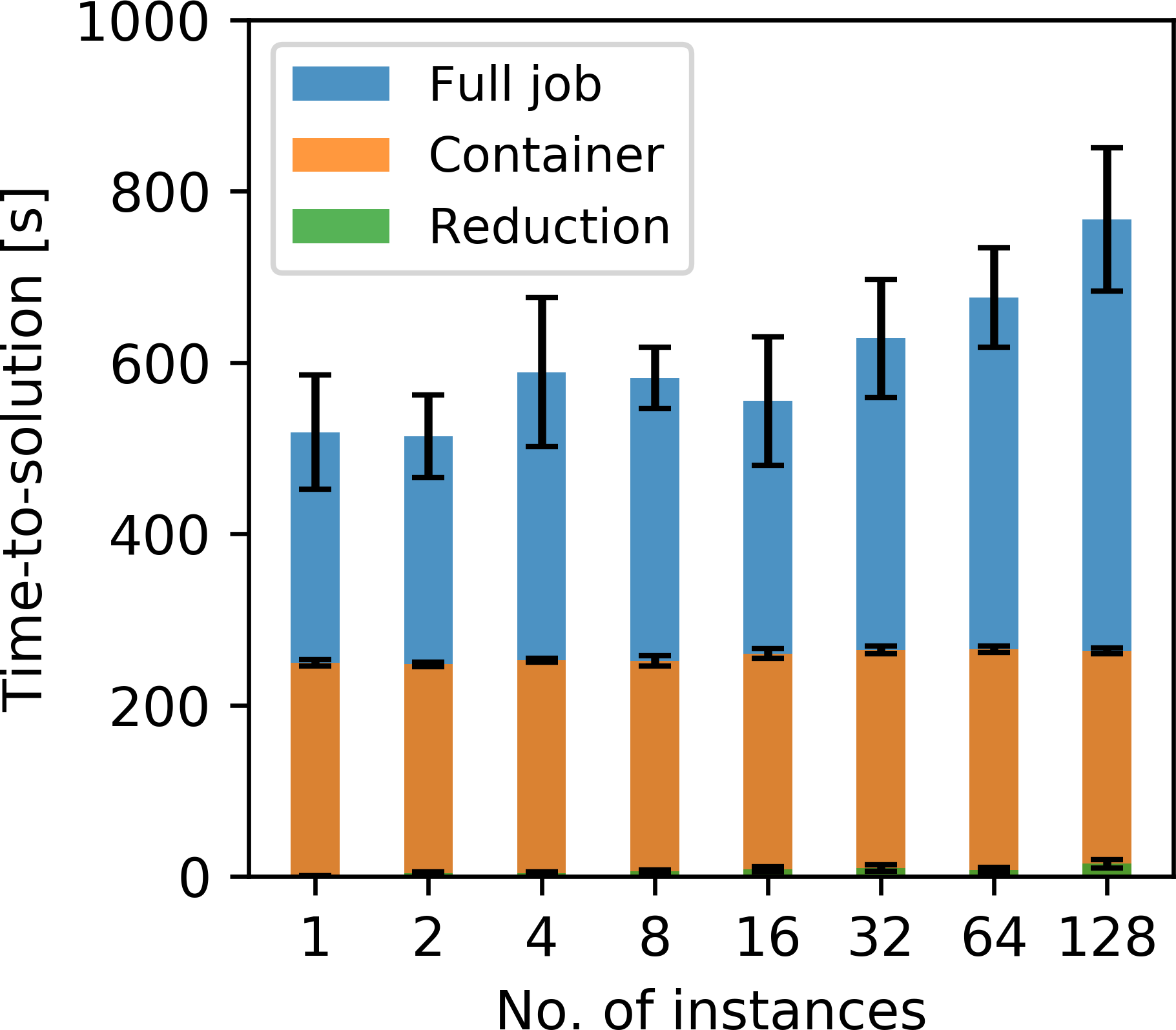


The timings ranging from a batch size of 1 to 128 are displayed in Figure 6a. The batch size corresponds to the number of parallel EC2 instances on which the jobs are executed. The time-to-solution consists of three components that make up the full runtime of each job:
The average time for AWS Batch to request and launch the EC2 instances and to start the Docker containers on those instances.
The runtime of the containers
The additional gradient reduction and image update time, which is given by the time interval between the termination of the AWS Batch job and the time stamp of the updated variable.
The sum of these components makes up the time-to-solution as shown in Figure 6a and each component is furthermore plotted separately in Figures 6b to 6d. All timings are the arithmetic mean over \(10\) individual runs and error bars represent the \(90\) percent confidence interval. The container runtimes of Figure 6c are the arithmetic mean of the individual container runtimes on each instance (varying from 1 to 128). The average container runtime is proportional to the cost of computing one individual gradient and is given by the container runtime times the price of the m4.4xlarge instance, which was $0.2748 per hour at the time of testing. No extra charges occurs for AWS Batch itself, i.e. for scheduling and launching the batch job.
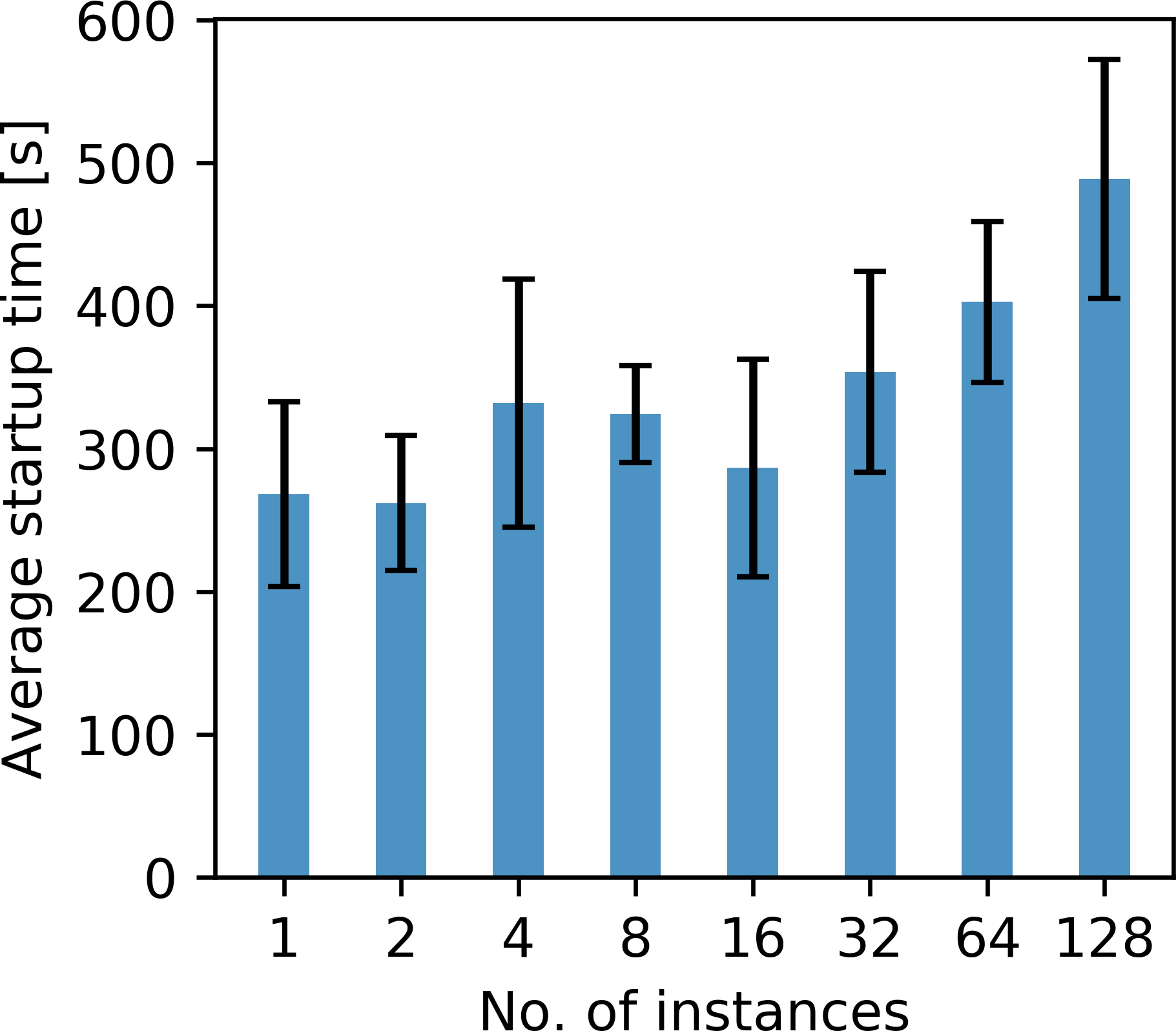
The timings indicate that the time-to-solution generally grows as the batch size, and therefore the number of containers per job, increases (Figure 6a). A close up inspection of the individual components that make up the total time-to-solution shows that this is mostly due to the increase of the startup time, i.e. the average time it takes AWS Batch to schedule and launch the EC2 instances for each job (Figure 6b). We found that AWS Batch does generally not start all instances of the array job at the same time, but instead in several stages, over the course of 1 to 3 minutes. The exact startup time depends on the batch size and therefore on the number of instances that need to be launched, but also on the availability of the instance within the AWS region. The combination of these factors leads to an increase of the average startup time for an increasing batch size, but also to a large variance of the startup time between individual runs. Users have no control over the startup time, but it is important to consider that no cost is incurred during this time period, as no EC2 instances are running while the individual containers remain in the queue.
The average container runtime, i.e. the average computation time of a single gradient, is fairly stable as the batch size increases (Figure 6c). This observation is consistent with the fact that each container of an AWS Batch array job runs as an individual Docker container and is therefore independent of the batch size. The container runtime increases only slightly for larger batch sizes and we observe a larger variance in some of the container runtimes. This variance stems from the fact that users do not have exclusive access to the EC2 instances on which the containers are deployed. Specifically, our containers run on m4.4xlarge instances, which have 8 cores (16 virtual CPUs) and 64 GB of memory. In practice, AWS deploys these instances on larger physical nodes and multiple EC2 instances (of various users) can run on the same node. We hypothesize that a larger batch size increases the chance of containers being deployed to a compute node that runs at full capacity, thus slightly increasing the average container runtime, as user do not have exclusive access to the full network capacity or memory bandwidth. The average container runtime also represents a lower bound on the time-to-solution (per iteration) that can be achieved by running the example as a classic (non-event driven) program on a fixed cluster. In this case there is no overhead from requesting EC2 instances, but other overhead may still occur, depending on how the source parallelization and gradient summation are implemented.

Finally, we also observe an increase in the additional gradient reduction time, i.e. the interval between the S3 timestamps of the final computed gradient \(\mathbf{g}_i\) and the updated image \(\mathbf{x}\). The batch size corresponds to the number of gradients that have to be summed before the gradient can be used to update the image. The event-driven gradient reduction invokes the summation process as soon as the first gradients are written to S3, so most gradients are already summed by the time the final worker finishes its gradient computation. For the event-driven gradient summation, the variance of the startup and container runtime is therefore advantageous, as it allows the summation to happen asynchronously. However, in our example, the time interval between the first two gradients being written to S3 (thus invoking the gradient reduction) and the final gradient being computed does not appear to be large enough to complete the summation of all gradients. Specifically, we see a general increase in the reduction time, as well as widening of the confidence interval. This variance is due to a non-deterministic component of our event-based gradient summation, resulting from a limitation of AWS Lambda. While users can specify a maximum number of messages that Lambda functions read from an SQS queue, it is not possible to force Lambda to read a minimum amount of two messages, resulting in most Lambda functions reading only a single message (i.e. one object name) from the queue. Since we need at least two messages to sum the corresponding gradients, we return the message to the queue and wait for a Lambda invocation with more than one message. The user has no control over this process and sometimes it takes several attempts until a Lambda function with multiple messages is invoked. The likelihood of this happening increases with a growing batch size, since a larger number of gradients need to be summed, which explains the increase of the reduction time and variance in Figure 6d.
Overall, the gradient summation and variable update finish within a few seconds after the last gradient is computed and the additional reduction time is small compared to the full time-to-solution. In our example, the startup time (Figure 6b) takes up the majority of the time-to-solution (Figure 6a), as it lies in the range of a few minutes and is in fact longer than the average container runtime of each worker (Figure 6c). However, the startup time is independent of the runtime of the containers, so the ratio of the startup time to the container runtime improves as the workload per container increases. For 3D imaging workloads, whose solution times for 3D wave equations are orders of magnitude higher than for two dimensions, it is therefore to be expected that the ratio between startup and computation time will shift considerably towards the latter. Indeed, in a follow-up application of our workflow to a 3D seismic data set on Microsoft Azure, the average container runtime to compute a gradient was 120 minutes, thus shifting the startup to computation time ratio to \(1:25\) (P. A. Witte et al., 2019a).
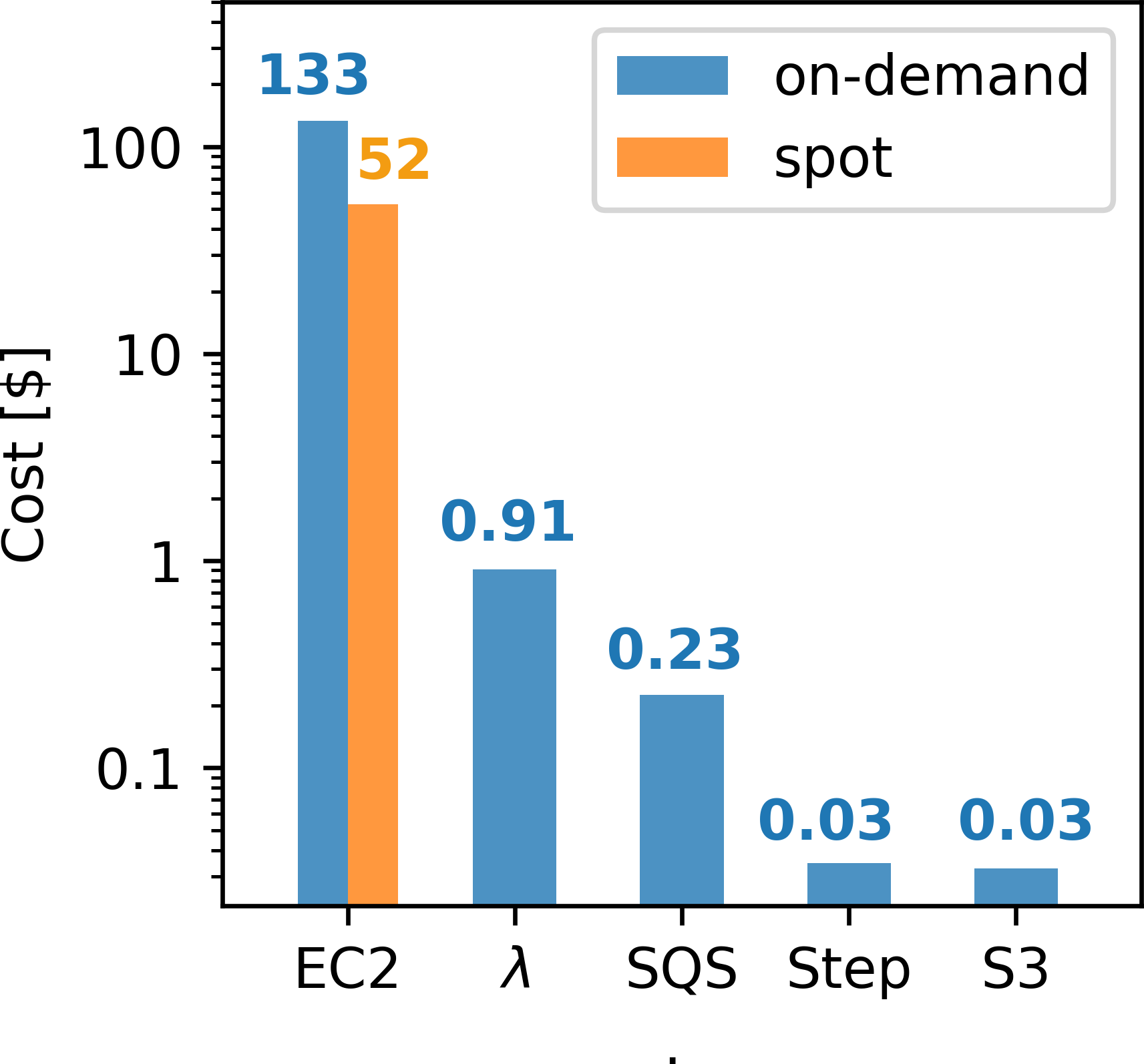
The cost of the batch job only depends on the container runtime and the batch size, but not on the startup time or reduction time. The cost for summing the gradients is given by the cumulative runtime of the Lambda functions, but is negligible compared to the EC2 cost for computing the gradients. This is illustrated in Figure 7a, which shows a cost breakdown of running our workflow for 30 iterations of stochastic gradient descent with a batch size of of 80, which corresponds to 1.8 epochs. The corresponding data misfit as a function of the iteration number is shown in Figure 7b. Similarly, SQS, Step Functions and S3 (i.e. the cost for storage and I/O) only contribute marginally to the full cost of running the imaging example, while the EC2 instances used by AWS Batch contribute by far the largest share. Using spot instances as opposed to on-demand instances for AWS Batch reduces the cost of our example by a factor of \(2.5\), but the prices of the remaining services are fixed. The seismic image after the final iteration number is shown in Figure 5b. In this example, every gradient was computed by AWS Batch on a single instance and a fixed number of threads, but in the subsequent section we analyze the scaling of runtime and cost as a function of the number of cores and EC2 instances. Furthermore, we will analyze in a subsequent example how the cost of running the gradient computations with AWS Batch compares to performing those computations on a fixed cluster of EC2 instances.
Strong scaling
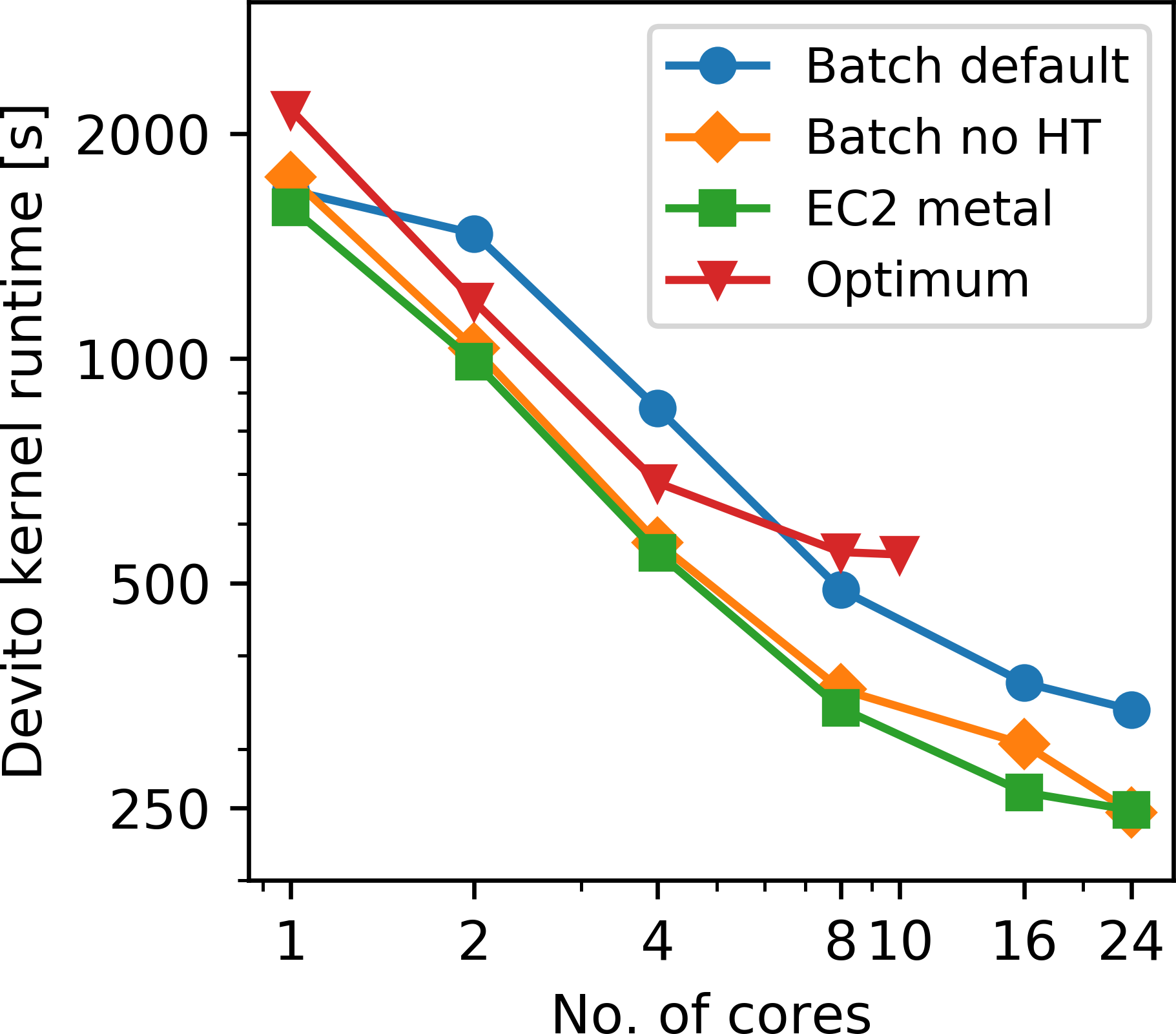
In the following set of experiments, we analyze the strong scaling behavior of our workflow for an individual gradient calculation, i.e. a gradient for a batch size of 1. For this, we consider a single gradient computation using AWS Batch and measure the runtime as a function of either the number of threads or the number of instances in the context of MPI-based domain decomposition. In the first experiment, we evaluate the vertical scaling behavior, i.e. we run the gradient computation on a single instance and vary the number of OpenMP threads. In contrast to the weak scaling experiment, we model wave propagation in the full domain (\(1,911 \times 10,789\) grid points), to ensure that the sub-domain of each worker is not too small when we use maximum number of threads.
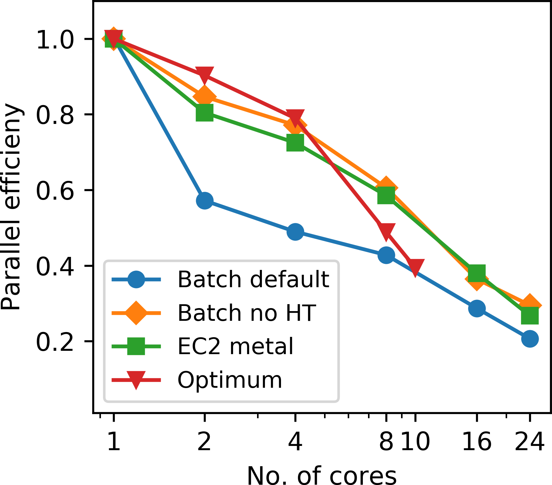
Since AWS Batch runs all jobs as Docker containers, we compare the runtimes with AWS Batch to running our application on a bare metal instance, in which case we have direct access to the compute node and run our code without any virtualization. All timings on AWS are performed on a r5.24xlarge EC2 instance, which is a memory optimized instance type that uses the Intel Xeon Platinum 8175M architecture (Appendix B). The 24xlarge instance has 96 virtual CPU cores (48 physical cores on 2 sockets) and 768 GB of memory. Using the largest possible instance of the r5 class, ensures that our AWS Batch job has exclusive access to the physical compute node, wile bare metal instances automatically give users exclusive access. We also include the Optimum HPC cluster in our comparison, a small research cluster at the University of British Columbia based on the Intel’s Ivy Bridge 2.8 GHz E5-2680v2 processor. Optimum has 2 CPUs per node and 10 cores per CPU. However, all OpenMP timings were conducted on single CPUs only, i.e. the maximum number of threads on each architecture corresponds to the maximum number of available cores per CPU (\(10\) on Optimum and \(24\) on the r5.24xlarge instances).
Figure 8a shows the comparison of the kernel runtimes on AWS and Optimum and Figure 8b displays the corresponding parallel efficiency. As expected, the r5 bare metal instance shows the best scaling, as it uses a newer architecture than Optimum and does not suffer from the virtualization overhead of Docker. We noticed that AWS Batch in its default mode uses hyperthreading (HT), even if we perform thread pinning and instruct AWS Batch to use separate physical cores. As of now, the only way to prevent AWS Batch from performing HT, is to modify the Amazon Machine Image (AMI) of the corresponding AWS compute environment. With HT disabled, the runtimes and speedups of AWS Batch are very close to the timings on the bare-metal instances, indicating that the overhead of Docker affects the runtimes and scaling of our memory-intensive application only marginally, which matches the findings of (Chung et al., 2016).
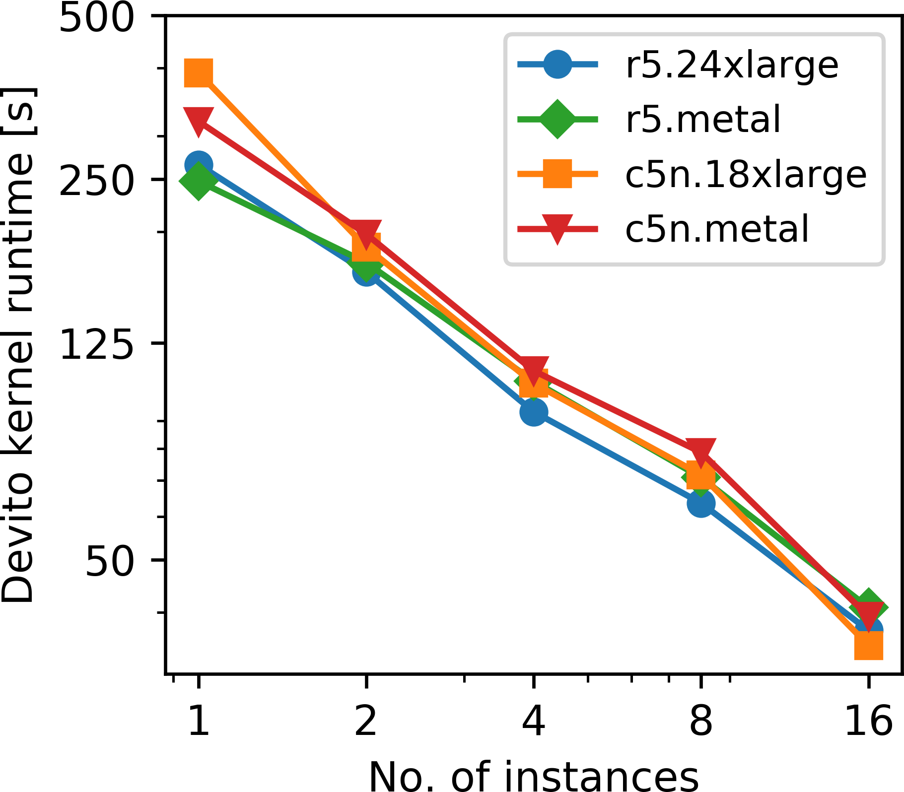
Next, we analyze the horizontal strong scaling behavior of running our application with AWS Batch. Once again, we consider the computation of one single gradient, but this time we vary the number of EC2 instances. We would like to emphasize that AWS Batch is used differently than in the weak scaling experiment, where AWS Batch was used to parallelize the sum over source locations and communication between workers of a separate jobs was not possible. Here, we submit a single workload (i.e. one gradient) as a multi-node AWS Batch job, in which case IP-based communication between instances is enabled. Since this involves distributed memory parallelism, we use domain decomposition based on message passing (MPI) to solve the wave equations on multiple EC2 instances (Valli and Quarteroni, 1999; “AWS documentation,” 2019f). The code with the corresponding MPI communication statements is automatically generated by the Devito compiler. Furthermore, we use multi-threading on each individual instance and utilize the maximum number of available cores per socket, which is 24 for the r5 instance and 18 for the c5n instance. To investigate the possible virtualization overhead of AWS Batch and Docker, we also conduct the same scaling experiments on clusters of EC2 bare metal instances, in which case our applications runs directly on the compute nodes without any form of virtualization.
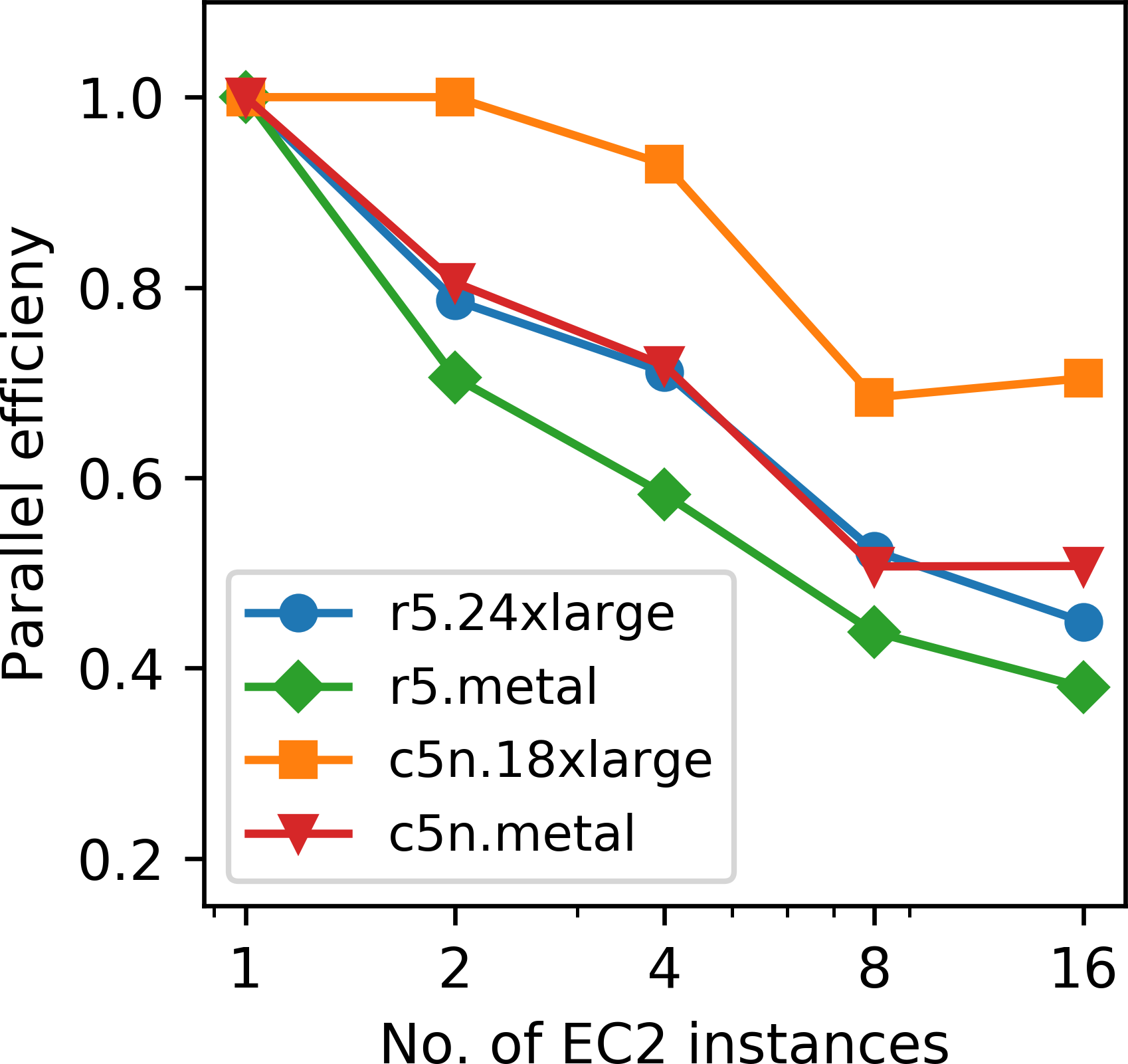
We compare the r5.24xlarge (and r5.metal) instances from the last section with Amazon’s recently introduced c5n HPC instance. Communication between AWS instances is generally based on ethernet and the r5 instances have up to 25 GBps networking performance. The c5n instance type uses Intel Xeon Platinum 8142M processors with up to 3.4 GHz architecture and according to AWS provides up to 100 GBps of network bandwidth. The network is based on a proprietary AWS technology called elastic fabric adapter (EFA), but AWS has not disclosed whether this technology is based on InfiniBand or Ethernet (“AWS elastic fabric adapter,” 2019). Figures 9a and 9b show the kernel runtimes and the corresponding parallel efficiency ranging from 1 to 16 instances for AWS Batch and on bare metal instances. The r5 instance has overall shorter runtimes than the c5n instance, since the former has 24 physical cores per CPU socket, while the c5n instance has 18. However, as expected, the c5n instance exhibits a better parallel efficiency than the r5 instance (in both batch mode and on bare metal), due to the better network performance. Interestingly, speedups and parallel efficiency of multi-node AWS Batch jobs are better than of the corresponding bare metal jobs, which is counter intuitive. To investigate this further, we measured the latency between two manually requested bare metal instances and two compute nodes assigned by AWS Batch and found that the latter set of instances have less than half the amount of latency (Appendix C). All nodes were requested in the same availability zone and EC2 placement group. This indicates that AWS possibly places instances for AWS Batch jobs closer to each other than manually requested EC2 instances, or that AWS Batch instances use a more efficient network gateway, but both of these explanations are purely speculative. Overall, the observed scaling and parallel efficiency of the AWS Batch jobs on both instances types are in the expected range of performance, as our application represents a strongly memory bound workload with an operational intensity of three FLOPs/Byte only, as shown in a roofline analysis of Devito’s generated code for acoustic modeling (M. Louboutin et al., 2019).

The timings given in Figure 9a are once again the pure kernel times for solving the PDEs, but a breakdown of the components that make up the total time-to-solution on the c5n instance is provided in Figure 9c. The job runtime is defined as the interval between the job creation time and the S3 time stamp of the computed gradient. As in our weak scaling test, this includes the time for AWS Batch to request and launch the EC2 instances, but excludes the gradient summation time, since we are only considering the computation of a single gradient. The container runtime is the runtime of the Docker container on the master node and includes the time it takes AWS Batch to launch the remaining workers and to establish an ssh connection between all instances/containers, which was the only supported communication protocol for AWS Batch at the time (“AWS documentation,” 2019f). Currently, AWS Batch requires this process to be managed by the user using a shell script that is run inside each container. The Python runtime in Figure 9c is defined as the runtime of our application on the main node and includes IO, memory allocation and code generation time. Our timings in Figure 9c show that the overhead from requesting instances and establishing a cluster, i.e. the difference between the Python and container runtime, is reasonable for a small number of instances, but grows significantly as the number instances is increased. Depending on the runtime of the application, the overhead thus takes up a significant amount of the time-to-solution, but for compute-heavy applications which run for one or multiple hours, this amount of overhead may still be acceptable. For 3D imaging applications that run for multiple hours, it is therefore to be expected that the ratio of application runtime to overhead will improve significantly.
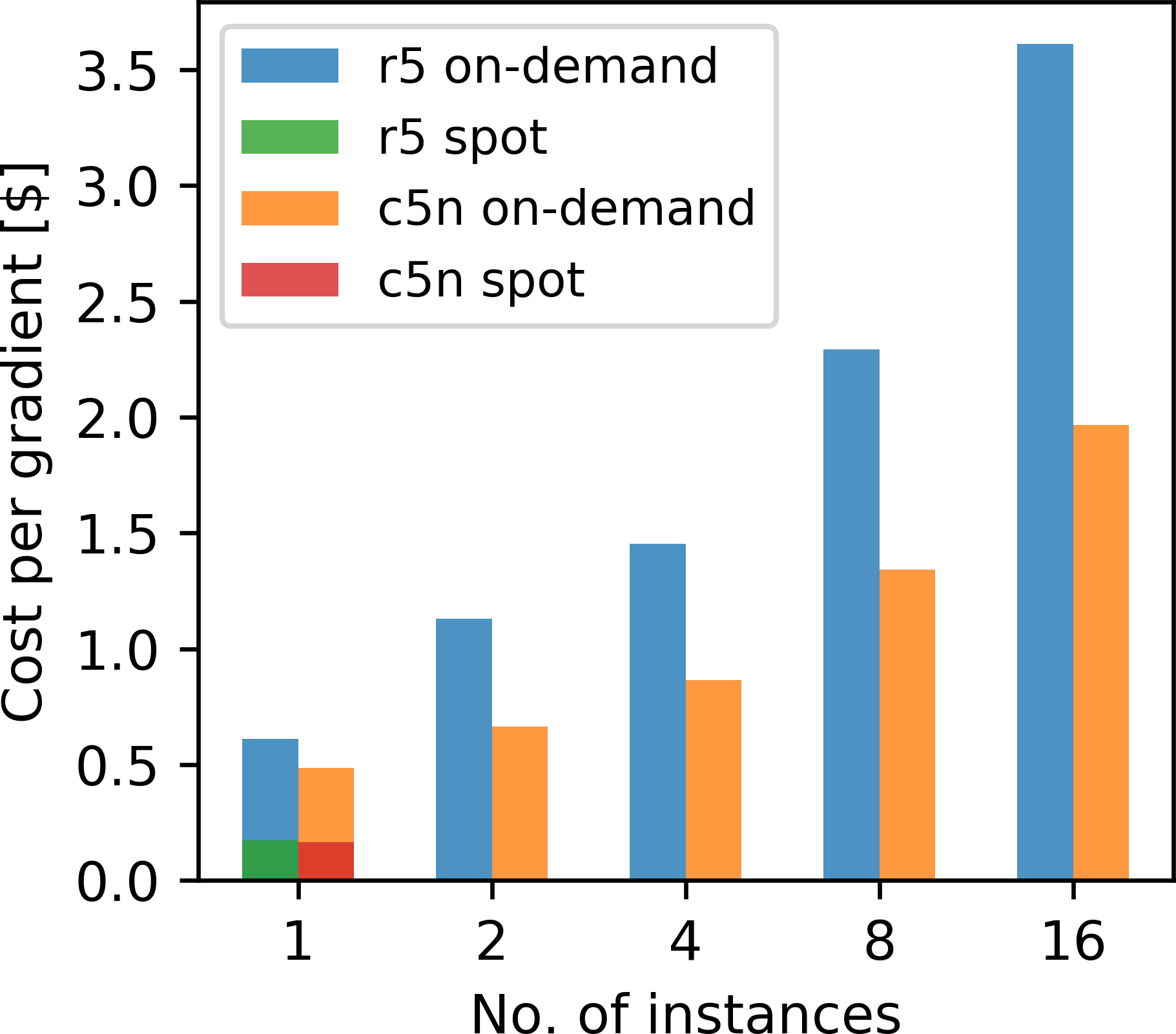
Figure 9d shows the cost for running our scaling test as a function of the cluster size. The cost is calculated as the instance price (per second) times the runtime of the container on the main node times the number of instances. The cost per gradient grows significantly with the number of instances, as the overhead from establishing an ssh connection to all workers increases with the cluster size. The communication overhead during domain decomposition adds an additional layer of overhead that further increases the cost for an increasing number of instances. This is an important consideration for HPC in the cloud, as the shortest time-to-solution does not necessarily correspond to the cheapest approach. Another important aspect is that AWS Batch multi-node jobs do not support spot instances (“AWS documentation,” 2019f). Spot instances allow users to access unused EC2 capacities at significantly lower price than at the on-demand price, but AWS Batch multi-node jobs are, or the time being, only supported with on-demand instances.
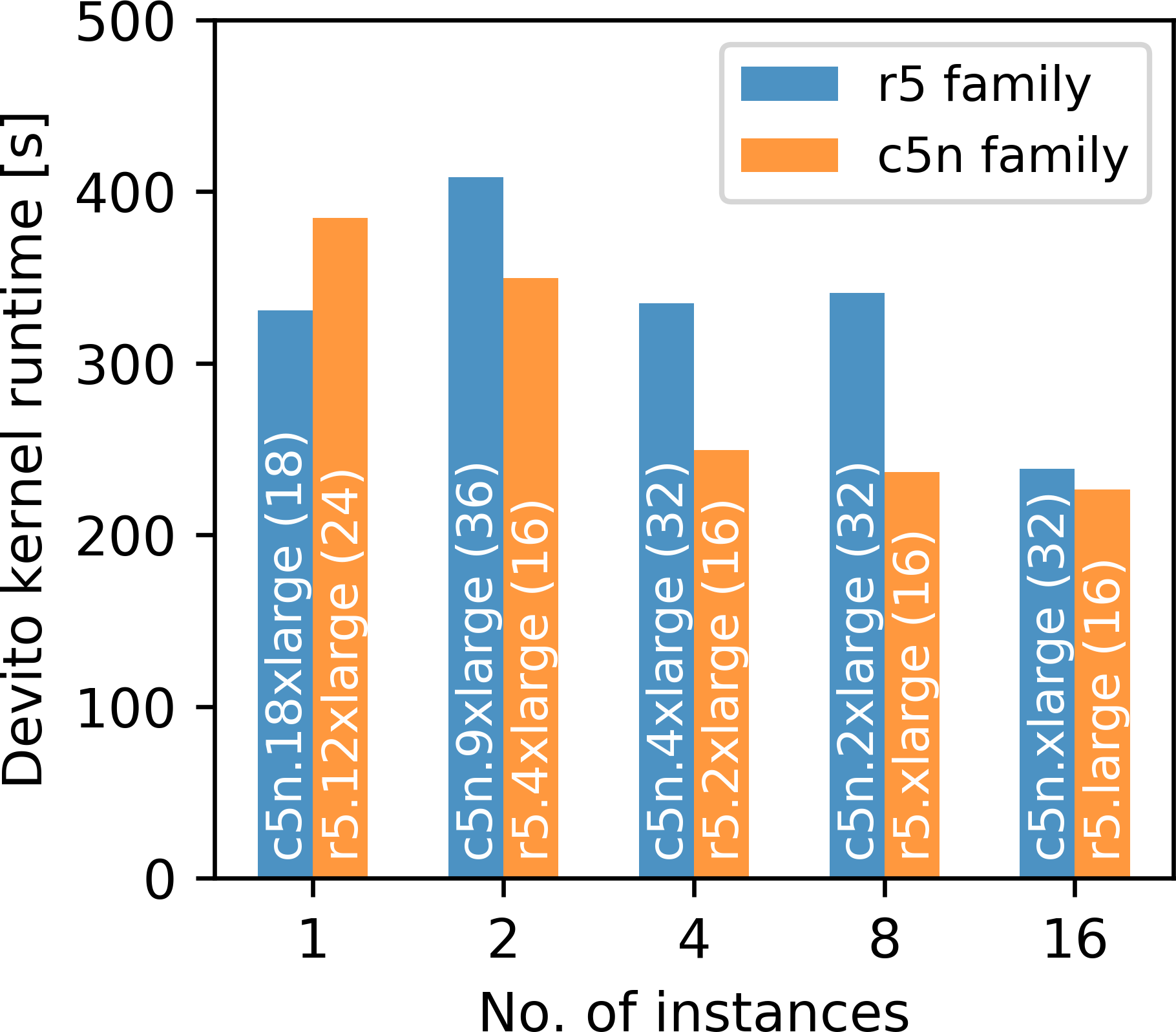

The scaling and cost analysis in Figures 9a – 9d was carried out on the largest instances of the respective instance types (r5.24xlarge and c5n.18xlarge) to guarantee exclusive access to the compute nodes and network bandwidth. Increasing the number of instances per run therefore not only increases the total number of available cores, but also the amount of memory. However, for computing a single gradient, the required amount of memory is fixed, so increasing the number of instances reduces the required amount of memory per instance, as wavefields are distributed among more workers. In practice, it therefore makes sense to chose the instance type based on the required amount of memory per worker, as memory is generally more expensive than compute. In our specific case, computing the gradient requires 170 GB of memory, which requires either a single r5.12xlarge instance or multiple smaller instances, which not only differ in the amount of memory, but also in the number of available CPU cores. We repeat our previous scaling test, but rather than using the same instance type in all runs, we choose the instance type based on the required amount of memory. Furthermore, for every instance type, we utilize the maximum amount of available cores using multi-threading with OpenMP. The kernel runtimes for an increasing number of instances is shown in Figure 10a. In each bar, we indicate which instance type was used, as well as the total number of cores across all instances. The corresponding costs for computing each gradient is shown in Figure 10a. Compared to the previous example, we observe that using 16 small on-demand instances leads to a lower cost than using a single more expensive large instance, but that using a single instance ultimately remains the most cost-effective way of computing a gradient, due to the possibility to utilize spot instances. An additional pricing model offered by AWS are reserved instances, which are EC2 instances that can be purchased at rates similar to spot prices if reserved for a minimum period of one year (“Amazon EC2 reserved instances pricing,” 2019). However, this pricing model is unsuitable for our event-driven approach, as users cannot save costs by minimizing idle time, since instances are paid for in advance.
| Grid | CPU Sockets | Cores | Parallelization | Runtime [s] |
|---|---|---|---|---|
| \(1,911 \times 5,394\) | \(1\) | \(24\) | OpenMP | \(190.17 \pm 7.12\) |
| \(1,911 \times 10,789\) | \(1\) | \(24\) | OpenMP | \(378.94 \pm 13.57\) |
| \(1,911 \times 10,789\) | \(2\) | \(48\) | OpenMP | \(315.92 \pm 16.50\) |
| \(1,911 \times 10,789\) | \(2\) | \(48\) | OpenMP + MPI | \(249.13 \pm 5.22\) |
In terms of cost, our scaling examples underline the importance of choosing the EC2 instances for the AWS Batch jobs based on the total amount of required memory, rather than based on the amount of CPU cores. Scaling horizontally by using an increasingly large number of instances expectedly leads to a faster time-to-solution, but results in a significant increase of cost as well (Figure 9d). As shown in Figure 10b, this increase in cost can be avoided to some extent by choosing the instance size such that the total amount of memory stays approximately constant, but ultimately the restriction of not supporting spot instances makes multi-node batch jobs not attractive in scenarios where single instances provide sufficient memory to run a given application. In practice, it makes therefore sense to use single node/instance batch jobs and to utilize the full number of available cores on each instance. The largest EC2 instances of each type (e.g. r5.24xlarge, c5n.18xlarge) have two CPU sockets with shared memory, making it possible to run parallel programs using either pure multi-threading or a hybrid MPI-OpenMP approach. In the latter case, programs still run as a single Docker container, but within each container use MPI for communication between CPU sockets, while OpenMP is used for multithreading on each CPU. For our example, we found that computing a single gradient of the BP model with the hybrid MPI-OpenMP approach leads to a 20% speedup over the pure OpenMP program (Table 1), which correspondingly leads to 20% cost savings as well.
Cost comparison
One of the most important considerations of high performance computing in the cloud is the aspect of cost. As users are billed for running EC2 instances by the second, it is important to use instances efficiently and to avoid idle resources. In our specific application, gradients for different seismic source locations are computed by a pool of parallel workers, but as discussed earlier, computations do not necessarily complete at the same time. On a conventional cluster, programs with a MapReduce structure, are implemented based on a client-server model, in which the workers compute the gradients in parallel, while the master (the server) collects and sums the results. This means that the process has to wait until all gradients \(\mathbf{g}_i\) have been computed, before the gradient can be summed and used to update the image. This inevitably causes workers that finish their computations earlier than others to the sit idle. This is problematic when using a cluster of EC2 instances, where the number of instances are fixed, as users have to pay for idle resources. In contrast, the event-driven approach based on Lambda functions and AWS Batch automatically terminates EC2 instances of workers that have completed their gradient calculation, thus preventing resources from sitting idle.
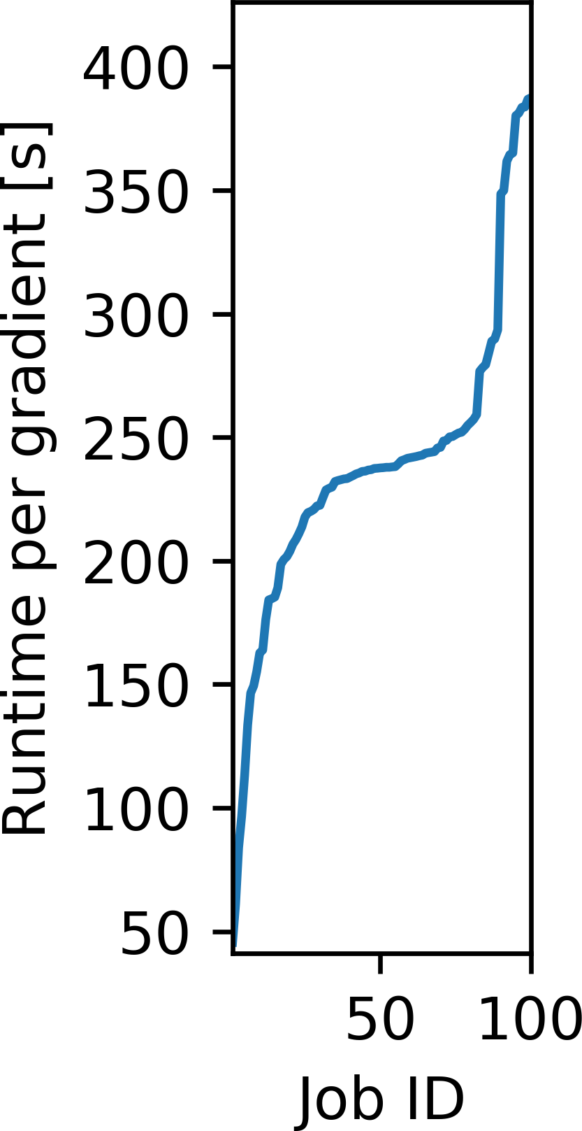
We illustrate the difference between the event-driven approach and using a fixed cluster of EC2 instances by means of a specific example. We consider our previous example of the BP synthetic model and compute the gradient \(\mathbf{g}_i\) for 100 random source locations and record the runtimes (Figure 11a). We note that most gradients take around 250 seconds to compute, but that the runtimes vary due to different domain sizes and varying EC2 capacity. We now model the idle time for computing these gradients on a cluster of EC2 instances as a function of the the number of parallel instances, ranging from 1 instance (fully serial) to 100 instances (fully parallel). For a cluster consisting of a single instance, the cumulative idle time is naturally zero, as the full workload is executed in serial. For more than one instance, we model the amount of time that each instance is utilized, assuming that the workloads are assigned on a first-come-first-served basis. The cumulative idle time \(t_\text{idle}\) is then given as the sum of the differences between the runtime of each individual instance \(t_i\) and the instance with the longest runtime: \[ \begin{equation} t_\text{idle} = \sum_{i=1}^{n_{\text{EC2}}} (\max\{t_i\} - t_i), \label{idletime} \end{equation} \] The cumulative idle time as a function of the cluster size \(n_\text{EC2}\) is plotted in Figure 11b. We note that the cumulative idle time generally increases with the cluster size, as a larger number of instances sit idle while waiting for the final gradient to be computed. On a cluster with 100 instances each gradient is computed by a separate instance, but all workers have to wait until the last worker finishes its computation (after approximately 387 seconds). In this case, the varying time-to-solutions of the individual gradients leads to a cumulative idle time of 248 minutes. Compared to the cumulative computation time of all gradients, which is 397 minutes, this introduces an overhead of more than 60 percent, if the gradients are computed on a cluster with 100 instances. The cumulative idle time is directly proportional to the cost for computing the 100 gradients, which is plotted on the right axis of Figure 11b. With AWS Batch, the cumulative idle time for computing the 100 gradients is zero, regardless of the number of parallel instances that AWS Batch has access to. Any EC2 instance that is not utilized anymore is automatically shut down by AWS Batch, so no additional cost other than the pure computation time of the gradients is invoked (“Announcing accelerated scale-down of AWS Batch managed compute environments,” 2019). A follow up case study of this work, found that the ratio of cumulative idle time to cumulative compute time (about 60 percent) also held true for a 3D seismic imaging example, in which the average container runtime was substanially longer than in the 2D (namely 120 minutes) (P. A. Witte et al., 2019a).

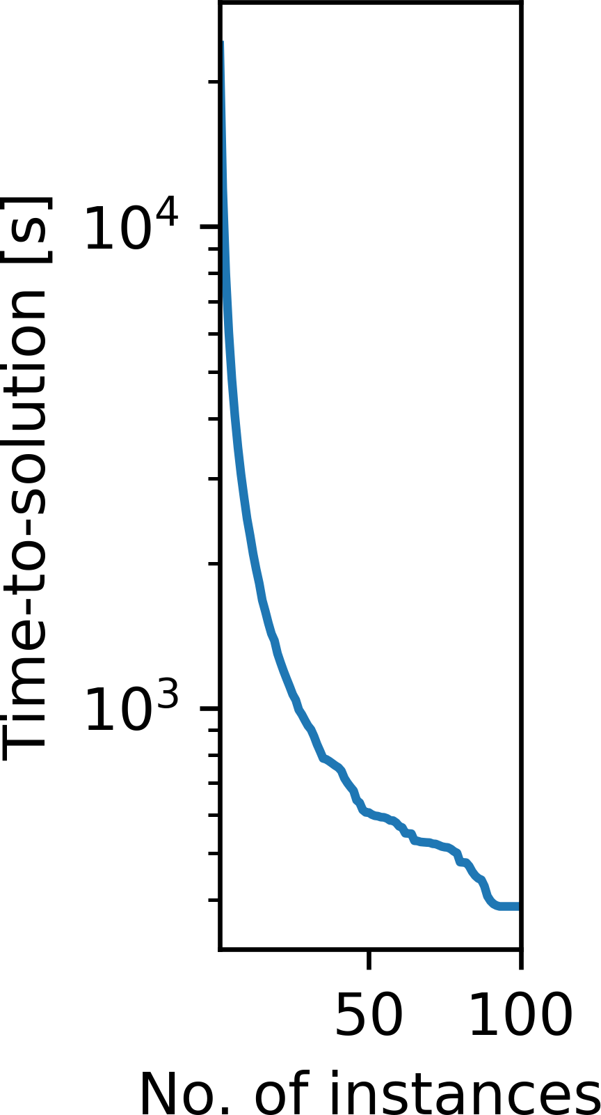
While computing the 100 gradients on an EC2 cluster with a small number of instances results in little cumulative idle time, it increases the overall time-to-solution, as a larger number of gradients have to be sequentially computed on each instance 11c. With AWS Batch this trade-off does not exist, as the cumulative idle time, and therefore the cost for computing a fixed workload, does not depend on the number of instances. However, it is to be expected that in practice the time-to-solution is somewhat larger for AWS Batch than for a fixed cluster of EC2 instances, as AWS Batch needs to request and launch EC2 instances for every new gradient computation.
Resilience
In the final experiment of our performance analysis, we analyze the resilience of our workflow and draw a comparison to running an MPI program on a conventional cluster of EC2 instances. Resilience is an important factor in high performance computing, especially for applications like seismic imaging, whose runtime can range from several hours to multiple days. In the cloud, the mean-time-between failures is typically much shorter than on comparable HPC systems (Jackson et al., 2010), making resilience potentially a prohibiting factor. Furthermore, using spot instances further increases the exposure to instance shut downs, as spot instances can be terminated at any point in time with a two minute warning.
Seismic imaging codes that run on conventional HPC clusters typically use MPI to parallelize the sum of the source indices and thus often leverage the User Level Fault Mitigation (ULFM) Standard (Bland et al., 2013) or the MVAPICH2 implementation of MPI, which includes built-in resilience (Chakraborty et al., 2018). Both MVAPICH2 and ULFM enable the continued execution of an MPI program after node/instance failures. In our event-driven approach, resilience in the cloud is naturally provided by using AWS Batch for the gradient computations, as each gradient is computed by a separate container. In case of exceptions, AWS Batch provides the possibility to automatically restart EC2 instances that have crashed, which allows the completion of programs with the initial number of nodes or EC2 instances.
We illustrate the effect of instance restarts by means of our previous example with the BP model (Figure 5a). Once again, we compute the gradient of the LS-RTM objective function for a batch size of 100 and record the runtimes without any instance/node failures. In addition to the default strategy for backpropagation, we compute the gradients using optimal checkpointing, in which case the average runtime per gradient increases from 5 minutes to 45 minutes, as a smaller memory footprint is traded for additional computations.

We then model the time that it takes to compute the 100 gradients for an increasing number of instance failures with and without restarts. We assume that the gradients are computed fully in parallel, i.e. on 100 parallel instances and invoke an increasing number of instance failures at randomly chosen times during the execution of program. Without instance restarts, we assign the workload of the failed instances to the workers of the remaining instances and model how long it takes complete the computations. With restarts, we add a two minute penalty to the failed worker and then restart the computation on the same instance. The two minute penalty represents the average amount of time it takes AWS Batch to restart a terminated EC2 instance and was determined experimentally.
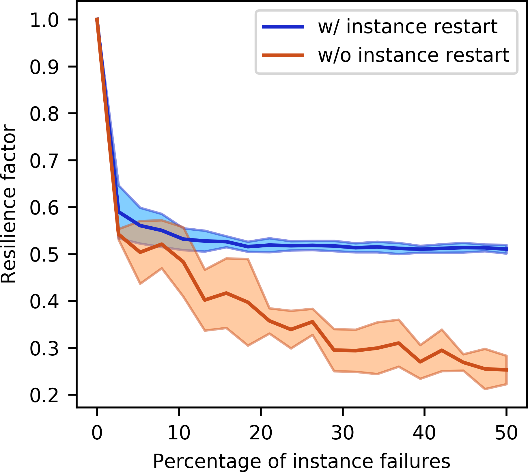
Figure 12 shows the ratio of the time-to-solution for computing the 100 gradients without events (i.e. without failures) to the modeled time-to-solution with events. This ratio is known as the resilience factor (Hukerikar et al., 2017) and provides a metric of how instance failures affect the time-to-solution and therefore the cost of running a given application in the cloud: \[ \begin{equation} r = \frac{\text{time-to-solution }_\text{ event-free}}{\text{time-to-solution }_\text{ event}} \label{resilience} \end{equation} \] Ideally, we aim for this factor being as close to 1 as possible, meaning that instance failures do not significantly increase the time-to-solution. Figures 12a and 12b compare the resilience factors with and without restarts for the two different backpropagation strategies, which represent programs of different runtimes. The resilience factor is plotted as a function of the percentage of instance failures and is the average of 10 realizations, with the standard deviation being depicted by the shaded colors. The plots show that the largest benefit from being able to restart instances with AWS Batch is achieved for long running applications (Figure 12b). The resilience factor with instance restarts approaches a value of 0.5, since in the worst case, the time-to-solution is doubled if an instance fails shortly before completing its gradient computation. Without being able to restart instances, the gradient computations need to be completed by the remaining workers, so the resilience factor continuously decreases as the failure percentage increases. For short running applications (Figure 12a), the overhead of restarting instances diminishes the advantage of instance restarts, unless a significant percentage of instances fail, which, however, is unlikely for programs that run in a matter of minutes. In fact, during our numerical experiments, we did not observed any spot-related shut-downs, as the runtime of our application was only in the order of five minutes. On the other hand, long running programs or applications with a large number of workers are much more likely to encounter instance shut downs and our experiment shows that these programs benefit from the automatic instance restarts of AWS Batch.
Discussion
The main advantage of an event-driven approach based on AWS Batch and Lambda functions for seismic imaging in the cloud is the automated management of computational resources by AWS. EC2 instances that are used for carrying out heavy computations, namely for solving large-scale wave equations, are started automatically in response to events, which in our case are Step Functions advancing the serverless workflow to the ComputeGradients state. Expensive EC2 instances are thus only active for the duration it takes to compute one element \(\mathbf{g}_i\) of the full or mini-batch gradient and they are automatically terminated afterwards. Summing the gradients and updating the variables (i.e. the seismic image) is performed on cheaper Lambda functions, with billing being again solely based on the execution time of the respective code and the utilized memory. The cost overhead introduced by Step Functions, SQS messages and AWS Batch is negligible compared to the cost of the EC2 instances that are required for the gradient computations, while cost savings from spot instances and eliminating idle EC2 instances lead to significant cost savings, as shown in our examples. With the benefits of spot instances (factor 2-3), avoidance of idle instances and the overhead of spinning clusters (factor 1.5-2), as well as improved resilience, we estimate that our event-driven workflow provides cost savings of up to an order of magnitude in comparison to using fixed clusters of (on-demand) EC2 instances.
A second alternative to running cloud applications on fixed EC2 clusters are in-between approaches based on a combination of EC2 instances, task-based workflow tools and auto-scaling. These approaches potentially benefit from the possibility to avoid containerization by using bare metal instances, while leveraging automatic up- and down-scaling of EC2 instances to save cost. However, workflow tools like AWS Batch or Step Functions are currently not available for EC2 clusters and thus need to be replicated by the user. Furthermore, any cluster-based workflows, even with auto-scaling, require at least a single EC2 instance to be permanently running, while our serverless approach makes it hypothetically possible to suspend tasks or workloads indefinitely without incurring any cost at all. Regarding performance, our analysis showed that Docker containerization did not lead to considerable performance impairments, while latency between EC2 instances assigned by AWS Batch was in fact smaller than latency between user-requested instances. Using batch processing to compute an embarrassingly parallel workload is not only advantageous in the cloud, but also on on-premise HPC systems, as parallel jobs that are broken into multiple smaller and shorter jobs are oftentimes processed faster by HPC schedulers than single large workloads. In addition to the improved flexibility regarding nested parallelization, this makes tasked-based asynchronous batch processing interesting in the setting of traditional HPC as well.
Another major advantage of our proposed serverless approach is the handling of resilience. Instead of running as a single program, our workflow is broken up into its individual components and expressed through Step Function states. Parallel programs based on MPI rely on not being interrupted by hardware failures during the entire runtime of the code, making this approach susceptible to resilience issues. Breaking a seismic imaging workflow into its individual components, with each component running as an individual (sub-) program and AWS managing their interactions, makes the event-driven approach inherently more resilient, as the runtime of individual workflow components is much shorter than the runtime of the full program, thus minimizing the exposure to instance failures. Computing an embarrassingly parallel workload with AWS Batch, rather than as a MPI-program, provides a natural layer of resilience, as AWS Batch processes each item from its queue separately on an individual EC2 instance and Docker container, but also includes the possibility of automatic instance restarts in the event of failures.
The most prominent disadvantage of the event-driven workflow is that EC2 instances have to be restarted by AWS Batch in every iteration of the workflow. In our performance analysis, we found that the overhead of requesting EC2 instances and starting the Docker container lies in the range of several minutes and depends on how many instances are requested per gradient. However, items that remain momentarily in the batch queue, do not incur any cost until the respective EC2 instance is launched. The overhead introduced by AWS Batch therefore only increases the time-to-solution, but does not affect the cost negatively. Due to the overhead of starting EC2 instances for individual computations, our proposed workflow is therefore applicable if the respective computations (e.g. computing gradients) are both embarrassingly parallel and take a long time to compute; ideally in the range of hours rather than minutes. We therefore expect that the advantages of our workflow will be even more prominent when applied to 3D seismic data sets, where computations are orders of magnitude more expensive than in 2D.
Our application, as expressed through AWS Step Functions, represents the structure of a generic gradient-based optimization algorithm and is therefore applicable to problems other than seismic imaging and full-waveform inversion. The design of our workflow lends itself to problems that exhibit a certain MapReduce structure, namely they consists of a computationally expensive, but embarrassingly parallel Map part, as well as a computationally cheaper to compute Reduce part. On the other hand, applications that rely on dense communications between workers or where the quantities of interest such as gradients or functions values are cheap to compute, are less suitable for this specific design. For example, deep convolutional neural networks (CNNs) exhibit mathematically a very similar problem structure to seismic inverse problems, but forward and backward evaluations of CNNs are typically much faster than solving forward and adjoint wave equations, even if we consider very deep networks like ResNet (He et al., 2016). Implementing training algorithms for CNNs as an event-driven workflow as presented here, is therefore excessive for the problem sizes that are currently encountered in deep learning, but might be justified in the future if the dimensionality of neural networks continues to grow.
The event-driven workflow presented in this work was specifically designed for AWS and takes advantage of specialized services for batch computing or event-driven computations that are available on this platform. However, in principle, it is possible to implement our workflow on other cloud platforms as well, as almost all of the utilized services have equivalent versions on Microsoft Azure or the Google Cloud Platform (Table 2) (“AWS to Azure services comparison,” 2019, 2019). Services for running parallel containerized workloads in the cloud, as well as event-driven cloud functions, which are the two main components of our workflow, are available on all platforms considered in our comparison. Furthermore, both Microsoft Azure as well as the GCP offer similar Python APIs as AWS for interfacing cloud services. We also speculate that, as cloud technology matures, services between different providers will likely grow more similar to each other. This is based on the presumption that less advanced cloud platforms will imitate services offered by major cloud providers in order to be competitive in the growing cloud market.
| Amazon Web Services | Microsoft Azure | Google Cloud Platform |
|---|---|---|
| Elastic Compute Cloud (EC2) | Azure Virtual Machines | Compute Engine |
| Simple Storage System (S3) | Azure Blob storage | Cloud Storage |
| AWS Batch | Azure Batch | Pipelines |
| Lambda Functions | Azure Functions | Cloud Functions |
| Step Functions | Logic Apps | N/A |
| Simple Message Queue (SQS) | Azure Queue Storage | Cloud Pub/Sub |
| Elastic File System (EFS) | Azure Files | Cloud Filestore (beta) |
Overall, our workflow and performance evaluation demonstrate that cost-competitive HPC in the cloud is possible, but requires a fundamental software re-design of the corresponding application. In our case, the implementation of an event-driven seismic imaging workflow was possible, as we leverage Devito for expressing and solving the underlying wave equations, which accounts for the major workload of seismic imaging. With Devito, we are able to abstract the otherwise complex implementation and performance optimization of wave equation solvers and take advantage of recent advances in automatic code generation. As Devito generates code for solving single PDEs, with the possibility of using MPI-based domain decomposition, we are not only able to leverage AWS Batch for the parallelization over source experiments, but can also take advantage of AWS Batch’s multi-node functionality to shift from data to model parallelism. In contrast, many seismic imaging codes are software monoliths, in which PDE solvers are enmeshed with IO routines, parallelization and manual performance optimization. Adapting codes of this form to the cloud is fundamentally more challenging, as it is not easily possible to isolate individual components such as a PDE solver for a single source location, while replacing the parallelization with cloud services. This illustrates that separation of concerns and abstract user interfaces are a prerequisite for porting HPC codes to the cloud such that the codes are able to take advantage of new technologies like object storage and event-driven computations. With a domain-specific language compiler, automatic code generation, high-throughput batch computing and serverless visual algorithm definitions, our workflow represents a true vertical integration of modern programming paradimgs into a framework for HPC in the cloud.
Conclusion
Porting HPC applications to the cloud using a lift and shift approach based on virtual clusters that emulate on-premise HPC clusters, is problematic as the cloud cannot offer the same performance and reliability as conventional clusters. Applications such as seismic imaging that are computationally expensive and run for a long time, are faced with practical challenges such as cost and resilience issues, which prohibit the cloud from being widely adapted for HPC tasks. However, the cloud offers a range of new technologies such as object storage or event-driven computations, that allow to address computational challenges in HPC in novel ways. In this work, we demonstrate how to adapt these technologies to implement a workflow for seismic imaging in the cloud that does not rely on a conventional cluster, but is instead based on serverless and event-driven computations. These tools are not only necessary to make HPC in the cloud financially viable, but also to improve the resilience of workflows. The code of our application is fully redesigned and uses a variety of AWS services as building blocks for the new workflow, thus taking advantage of AWS being responsible for resilience, job scheduling, and resource allocations. Our performance analysis shows that the resulting workflow exhibits competitive performance and scalability, but most importantly minimizes idle time on EC2 instances and cost and is inherently resilient. Our example therefore demonstrates that successfully porting HPC applications to the cloud is possible, but requires to carefully adapt the corresponding codes to to the new environment. This process is heavily dependent on the specific application and involves identifying properties of the underlying scientific problem that can be exploited by new technologies available in the cloud. Most importantly, it requires that codes are modular and designed based on the principle of separation of concerns, thus making this transition possible.
Acknowledgments
The authors would like to acknowledge Dr. Fabio Luporini and Dr. Gerard J. Gorman (Imperial College London) for their work on Devito and their valuable input on the performance evaluation. This research was funded by the Georgia Research Alliance and the Georgia Institute of Technology.
Appendix
Wave equations
In the context of seismic imaging, the forward modeling operator \(\mathcal{F}\) denotes the (linearized) Born scattering operator (Claerbout, 1992): \[ \begin{equation} \mathcal{F}(\mathbf{\delta m}, \mathbf{q}) = -\mathbf{P}_r \mathbf{A}(\mathbf{m})^{-1} \frac{\partial^2}{\partial t^2}\mathbf{A}(\mathbf{m})^{-1} \mathbf{P}_s^\top \mathbf{q} \odot \delta \mathbf{m} \label{nonlinear_modeling} \end{equation} \] where the vector \(\mathbf{\delta m}\) denotes the (vectorized) seismic image, \(\mathbf{m}\) is the (known) velocity model, \(\mathbf{q}\) is the time signature of the seismic source and \(\odot\) represents element-wise multiplication. The matrices \(\mathbf{P}_s\) and \(\mathbf{P}_r\) are source and receiver projection operators, which sample the time-dependent wavefield at the source/receiver locations, while their adjoint correspondingly injects data back into the model. In this work, we choose the operator \(\mathbf{A}(\mathbf{m})\) to be the acoustic wave equation with constant density as given by: \[ \begin{equation} \underbrace{\Bigg(\mathbf{m} \odot \frac{\partial^2}{\partial t^2} - \mathbf{L} \Bigg)}_{\mathbf{A}(\mathbf{m})} \mathbf{u} = \mathbf{P}_s^\top \mathbf{q}. \label{acoustic_we} \end{equation} \] The operator \(\mathbf{L}\) denotes the Laplacian, which we discretize using finite differences (FD) and \(\mathbf{u}\) is the vectorized wavefield for all time steps. Computing the action of the inverse of \(\mathbf{A}(\mathbf{m})\) corresponds to solving this linear system using FD time stepping. In general, other representations of the physics or discretizations, such as finite elements, are possible as well. Discretization of the second time derivative with a second order FD stencil leads to the following time stepping scheme, which computes the wavefield \(\mathbf{u}^n\) for subsequent time steps \(n=1, .., n_t\): \[ \begin{equation} \mathbf{u}^{n+1} = \Bigg[2 + \frac{\Delta t^2}{\mathbf{m}} \odot \mathbf{L}\Bigg] \mathbf{u}^n - \mathbf{u}^{n-1} + \frac{\Delta t^2}{\mathbf{m}} \odot \mathbf{P}_{s}^\top\mathbf{q}^{n+1} \label{time_stepping} \end{equation} \] The scheme is initialized with \(\mathbf{u}^0 = \mathbf{u}^1 = 0\). In practice, the time stepping scheme also includes an additional dampingterm to mimic wave propagation in an unbounded medium. In our framework, we implement and solve forward and adjoint (linearized) wave equations with Devito and a detailled description of the implementation is given in (Louboutin et al., 2017, 2018).
Computational resources
Table 3 provides an overview of the AWS EC2 instances used in our performance analysis, including their respective CPU architectures. EC2 instances of a fixed instance type (such as r5 or c5n) have the same architecture for different sizes (e.g. 2xlarge, 4xlarge), as those instances run on the same hardware.
| Instance | Architecture | (v)CPUs | Cores/socket | Sockets | Memory (GB) |
|---|---|---|---|---|---|
| m4.4xlarge | Intel Xeon E5-2686 v4 @ 2.30GHz | 16 | 8 | 1 | 64 |
| r5.12xlarge | Intel Xeon Platinum 8175M @ 2.50 GHz | 48 | 24 | 1 | 384 |
| r5.24xlarge | Intel Xeon Platinum 8175M @ 2.50 GHz | 96 | 24 | 2 | 768 |
| c5n.9xlarge | Intel Xeon Platinum 8124M @ 3.00 GHz | 36 | 18 | 1 | 384 |
| c5n.12xlarge | Intel Xeon Platinum 8142M @ 3.00 GHz | 72 | 18 | 2 | 768 |
| r5.metal | Intel Xeon Platinum 8175M @ 2.50 GHz | 96 | 24 | 2 | 768 |
| Optimum | Intel Xeon E5-2680 v2 @ 2.80GHz | 20 | 10 | 2 | 256 |
Latency
| Instance | Latency AWS Batch | Latency bare metal |
|---|---|---|
| min/avg/max/mdev [ms] | min/avg/max/mdev [ms] | |
| r5 | 0.068/0.073/0.095/0.009 | 0.142/0.193/0.453/0.088 |
| c5n | 0.073/0.087/0.106/0.013 | 0.082/0.151/0.173/0.038 |
Table 4 provides a comparison of latencies between two EC2 instances that were launched for a multi-node AWS Batch job and two manually requested EC2 bare metal instances of the corresponding type. All instances were requested in the us-east-1a zone within an EC2 cluster placement group. Latencies were obtained via the ping command and represent the minimum, average, maximum value and the standard deviation of 20 56 byte packages.
References
Abdelkhalek, R., Calandra, H., Coulaud, O., Roman, J., and Latu, G., 2009, Fast seismic modeling and reverse time migration on a GPU cluster: In 2009 international conference on high performance computing simulation (pp. 36–43). doi:10.1109/HPCSIM.2009.5192786
Amazon EC2 reserved instances pricing: 2019, https://aws.amazon.com/ec2/pricing/reserved-instances/pricing/ ; Amazon Web Services. Retrieved January 8, 2020, from
Announcing accelerated scale-down of AWS Batch managed compute environments: 2019, https://aws.amazon.com/about-aws/whats-new/2017/10/announcing-accelerated-scale-down-of-aws-batch-managed-compute-environments/; Amazon Web Services. Retrieved June 21, 2019, from
AWS documentation: Amazon EC2 instance types: 2019a, https://aws.amazon.com/ec2/instance-types/; Amazon Web Services User Guide. Retrieved July 30, 2019, from
AWS documentation: Amazon Elastic Compute Cloud: 2019b, https://docs.aws.amazon.com/batch/latest/userguide/what-is-batch.html; Amazon Web Services User Guide. Retrieved July 26, 2019, from
AWS documentation: Amazon EMR: 2019c, https://docs.aws.amazon.com/emr/latest/ManagementGuide/emr-overview.html; Amazon Web Services User Guide. Retrieved August 12, 2019, from
AWS documentation: Amazon Simple Queue Service: 2019d, https://docs.aws.amazon.com/AmazonS3/latest/dev/Welcome.html; Amazon Web Services User Guide. Retrieved July 25, 2019, from
AWS documentation: Amazon Simple Storage Service: 2019e, https://docs.aws.amazon.com/AmazonS3/latest/dev/Welcome.html; Amazon Web Services User Guide. Retrieved July 25, 2019, from
AWS documentation: AWS Batch - multi node parallel jobs: 2019f, https://docs.aws.amazon.com/batch/latest/userguide/multi-node-parallel-jobs.html; Amazon Web Services User Guide. Retrieved July 29, 2019, from
AWS documentation: AWS Batch: 2019g, https://aws.amazon.com/ec2/; Amazon Web Services User Guide. Retrieved March 19, 2019, from
AWS documentation: AWS Lambda: 2019h, https://aws.amazon.com/lambda/; Amazon Web Services User Guide. Retrieved June 1, 2019, from
AWS documentation: AWS Step Functions: 2019i, https://aws.amazon.com/step-functions/; Amazon Web Services User Guide. Retrieved July 26, 2019, from
AWS documentation: How spot instances work: 2019j, https://docs.aws.amazon.com/AWSEC2/latest/UserGuide/how-spot-instances-work.html; Amazon Web Services: User Guide for Linux Instances. Retrieved March 21, 2019, from
AWS elastic fabric adapter: 2019, https://aws.amazon.com/hpc/efa/; Amazon Web Services User Guide. Retrieved March 9, 2020, from
AWS enterprise customer success stories: 2019, https://aws.amazon.com/solutions/case-studies/enterprise; Amazon Web Services Case Studies. Retrieved March 19, 2019, from
AWS High Performance Computing: 2019, https://aws.amazon.com/hpc/; Amazon Web Services User Guide. Retrieved June 5, 2019, from
AWS Nitro system: 2019, https://aws.amazon.com/ec2/nitro/; Amazon Web Services User Guide. Retrieved January 6, 2020, from
AWS to Azure services comparison: 2019, https://docs.microsoft.com/en-us/azure/architecture/aws-professional/services; Microsoft Azure Documentation. Retrieved July 30, 2019, from
Beck, A., and Teboulle, M., 2009, A fast iterative shrinkage-thresholding algorithm for linear inverse problems: SIAM Journal on Imaging Sciences, 2, 183–202.
Billette, F., and Brandsberg-Dahl, S., 2005, The 2004 BP velocity benchmark.: In 67th Annual International Meeting, EAGE, Expanded Abstracts (p. B035). EAGE.
Bland, W., Bouteiller, A., Herault, T., Bosilca, G., and Dongarra, J., 2013, Post-failure recovery of MPI communication capability: Design and rationale: The International Journal of High Performance Computing Applications, 27, 244–254.
Boto 3 documentation: 2019, https://boto3.amazonaws.com/v1/documentation/api/latest/index.html#; Amazon Web Services. Retrieved July 26, 2019, from
Bottou, L., 2010, Large-scale machine learning with stochastic gradient descent: In Proceedings of 15th international conference on computational statistics (cOMPSTAT’2010) (pp. 177–186). Springer.
Chakraborty, S., Laguna, I., Emani, M., Mohror, K., Panda, D. K., Schulz, M., and Subramoni, H., 2018, EReinit: Scalable and efficient fault-tolerance for bulk-synchronous mPI applications: Concurrency and Computation: Practice and Experience, n/a, e4863. doi:10.1002/cpe.4863
Chung, M. T., Quang-Hung, N., Nguyen, M.-T., and Thoai, N., 2016, Using Docker in high performance computing applications: In 2016 iEEE sixth international conference on communications and electronics (iCCE) (pp. 52–57). IEEE.
Claerbout, J., 1992, Earth soundings analysis: Processing versus inversion: Blackwell Scientific Publications. Retrieved from https://books.google.ca/books?id=ws1qQgAACAAJ
Dean, J., and Ghemawat, S., 2008, MapReduce: Simplified data processing on large clusters: Communications of the ACM, 51, 107–113.
Docker: 2019, https://www.docker.com/; Docker. Retrieved July 26, 2019, from
Dong, S., Cai, J., Guo, M., Suh, S., Zhang, Z., Wang, B., and Li, Z., 2012, Least-squares reverse time migration: Towards true amplitude imaging and improving the resolution: In 82nd annual international meeting, sEG, expanded abstracts (pp. 1–5). doi:10.1190/segam2012-1488.1
Fletcher, R., and Reeves, C. M., 1964, Function minimization by conjugate gradients: The Computer Journal, 7, 149–154.
Friedman, A., and Pizarro, A., 2017, Building high-throughput genomics batch workflows on AWS:. https://aws.amazon.com/blogs/compute/building-high-throughput-genomics-batch-workflows-on-aws-introduction-part-1-of-4/; AWS Compute Blog.
Furse, C. M., 1998, Faster than Fourier-ultra-efficient time-to-frequency domain conversions for FDTD: In Institute of electrical and electronics engineers (iEEE): Antennas and propagation society international symposium (Vol. 1, pp. 536–539 vol.1). doi:10.1109/APS.1998.699196
Garfinkel, S. L., 2007, An evaluation of Amazon’s grid computing services: EC2, S3, and SQS: In Harvard computer science group technical report tR-08-07.
Google Cloud Platform for AWS professionals: 2019, https://cloud.google.com/docs/compare/aws/; Google Cloud Documentation. Retrieved July 30, 2019, from
Griewank, A., and Walther, A., 2000, Algorithm 799: Revolve: An implementation of checkpointing for the reverse or adjoint mode of computational differentiation: Association for Computing Machinery (ACM) Transactions on Mathematical Software, 26, 19–45. doi:10.1145/347837.347846
Gropp, W., Gropp, W. D., Lusk, A. D. F. E. E., Lusk, E., and Skjellum, A., 1999, Using MPI: Portable parallel programming with the message-passing interface: (Vol. 1). MIT press.
Gupta, A., and Milojicic, D., 2011, Evaluation of HPC applications on cloud: In 2011 sixth open cirrus summit (pp. 22–26). IEEE.
He, K., Zhang, X., Ren, S., and Sun, J., 2016, Deep residual learning for image recognition: In Proceedings of the iEEE conference on computer vision and pattern recognition (pp. 770–778).
Hukerikar, S., Ashraf, R. A., and Engelmann, C., 2017, Towards new metrics for high-performance computing resilience: In Proceedings of the 2017 workshop on fault-tolerance for hPC at extreme scale (pp. 23–30). ACM.
Iosup, A., Ostermann, S., Yigitbasi, M. N., Prodan, R., Fahringer, T., and Epema, D., 2011, Performance analysis of cloud computing services for many-tasks scientific computing: IEEE Transactions on Parallel and Distributed Systems, 22, 931–945. doi:10.1109/TPDS.2011.66
Iterating a loop using Lambda: 2018, https://docs.aws.amazon.com/step-functions/latest/dg/tutorial-create-iterate-pattern-section.html; AWS Step Functions Developer Guide. Retrieved June 12, 2018, from
Jackson, K. R., Muriki, K., Ramakrishnan, L., Runge, K. J., and Thomas, R. C., 2011, Performance and cost analysis of the supernova factory on the Amazon AWS cloud: Scientific Programming, 19, 107–119.
Jackson, K. R., Ramakrishnan, L., Muriki, K., Canon, S., Cholia, S., Shalf, J., … Wright, N. J., 2010, Performance analysis of high performance computing applications on the Amazon Web Services cloud: In 2010 iEEE second international conference on cloud computing technology and science (pp. 159–168). IEEE.
Joyner, D., Čertík, O., Meurer, A., and Granger, B. E., 2012, Open source computer algebra systems: SymPy: Association for Computing Machinery (ACM) Communications in Computer Algebra, 45, 225–234. doi:10.1145/2110170.2110185
Kingma, D. P., and Ba, J., 2014, Adam: A method for stochastic optimization: ArXiv E-Prints, abs/1412.6980. Retrieved from https://arxiv.org/abs/1412.6980
Kotas, C., Naughton, T., and Imam, N., 2018, A comparison of Amazon Web Services and Microsoft Azure cloud platforms for high performance computing: In 2018 iEEE international conference on consumer electronics (iCCE) (pp. 1–4). IEEE.
Louboutin, M., Lange, M., Luporini, F., Kukreja, N., Witte, P. A., Herrmann, F. J., … Gorman, G. J., 2019, Devito (v3.1.0): An embedded domain-specific language for finite differences and geophysical exploration: Geoscientific Model Development, 12, 1165–1187. doi:10.5194/gmd-12-1165-2019
Louboutin, M., Witte, P., Lange, M., Kukreja, N., Luporini, F., Gorman, G., and Herrmann, F. J., 2017, Full-waveform inversion, Part 1: Forward modeling: The Leading Edge, 36, 1033–1036. doi:10.1190/tle36121033.1
Louboutin, M., Witte, P., Lange, M., Kukreja, N., Luporini, F., Gorman, G., and Herrmann, F. J., 2018, Full-waveform inversion, Part 2: Adjoint modeling: The Leading Edge, 37, 69–72. doi:10.1190/tle37010069.1
Luporini, F., Lange, M., Louboutin, M., Kukreja, N., Hückelheim, J., Yount, C., … Herrmann, F. J., 2018, Architecture and performance of Devito, a system for automated stencil computation: To Be Published in ACM Transactions on Mathematical Software. Retrieved from https://arxiv.org/abs/1807.03032
Mehrotra, P., Djomehri, J., Heistand, S., Hood, R., Jin, H., Lazanoff, A., … Biswas, R., 2016, Performance evaluation of Amazon Elastic Compute Cloud for NASA high-performance computing applications: Concurrency and Computation: Practice and Experience, 28, 1041–1055.
Mohammadi, M., and Bazhirov, T., 2018, Comparative benchmarking of cloud computing vendors with high performance LINPACK: In Proceedings of the 2nd international conference on high performance compilation, computing and communications (hP3C-2018) (pp. 1–5). ACM.
Napper, J., and Bientinesi, P., 2009, Can cloud computing reach the Top500? In Proceedings of the combined workshops on unconventional high performance computing workshop plus memory access workshop (uCHPC-mAW ’09) (pp. 17–20). ACM. doi:10.1145/1531666.1531671
Nesterov, Y., 2018, Lectures on convex optimization: (Vol. 137). Springer.
Nocedal, J., and Wright, S., 2006, Numerical optimization: Springer Science & Business Media.
Peters, B., Smithyman, B. R., and Herrmann, F. J., 2019, Projection methods and applications for seismic nonlinear inverse problems with multiple constraints: GEOPHYSICS, 84, R251–R269. doi:10.1190/geo2018-0192.1
Pratt, R. G., 1999, Seismic waveform inversion in the frequency domain, part 1: Theory and verification in a physical scale model: Geophysics, 64, 888–901. doi:10.1190/1.1444597
Rad, J., Ragab, A., and Damodar, A., 2018, Building a tightly coupled molecular dynamics workflow with multi-node parallel jobs in AWS Batch:. https://aws.amazon.com/blogs/compute/building-a-tightly-coupled-molecular-dynamics-workflow-with-multi-node-parallel-jobs-in-aws-batch/; AWS Compute Blog.
Rad, P., Chronopoulos, A., Lama, P., Madduri, P., and Loader, C., 2015, Benchmarking bare metal cloud servers for HPC applications: In 2015 iEEE international conference on cloud computing in emerging markets (cCEM) (pp. 153–159). IEEE.
Ramakrishnan, L., Canon, R. S., Muriki, K., Sakrejda, I., and Wright, N. J., 2012, Evaluating interconnect and virtualization performance for high performance computing: ACM SIGMETRICS Performance Evaluation Review, 40, 55–60.
Ruthotto, L., and Haber, E., 2018, Deep neural networks motivated by partial differential equations: CoRR, abs/1804.04272. Retrieved from http://arxiv.org/abs/1804.04272
Ruthotto, L., Treister, E., and Haber, E., 2017, jInv–a flexible Julia package for PDE parameter estimation: SIAM Journal on Scientific Computing, 39, S702–S722. doi:10.1137/16M1081063
Sadooghi, I., Martin, J. H., Li, T., Brandstatter, K., Maheshwari, K., de Lacerda Ruivo, T. P. P., … Raicu, I., 2017, Understanding the performance and potential of cloud computing for scientific applications: IEEE Transactions on Cloud Computing, 5, 358–371. doi:10.1109/TCC.2015.2404821
Scheuner, J., and Leitner, P., 2018, A cloud benchmark suite combining micro and applications benchmarks: In Companion of the 2018 aCM/SPEC international conference on performance engineering (pp. 161–166). Association for Computing Machinery. doi:10.1145/3185768.3186286
Seismic processing and imaging:, 2019, https://www.pgs.com/imaging/services/processing-and-imaging/.
Silva, C. D., and Herrmann, F. J., 2017, A unified 2D/3D large-scale software environment for nonlinear inverse problems: ACM Transactions on Mathematical Software, 45, 7:1–7:35.
StarCluster: 2019, http://star.mit.edu/cluster/; Massachusetts Institute of Technology. Retrieved June 5, 2019, from
Symes, W. W., Sun, D., and Enriquez, M., 2011, From modelling to inversion: Designing a well-adapted simulator: Geophysical Prospecting, 59, 814–833. doi:10.1111/j.1365-2478.2011.00977.x
Tarantola, A., 1984, Inversion of seismic reflection data in the acoustic approximation: Geophysics, 49, 1259. doi:10.1190/1.1441754
Valenciano, A. A., 2008, Imaging by wave-equation inversion: PhD thesis,. Stanford University.
Valli, A., and Quarteroni, A., 1999, Domain decomposition methods for partial differential equations: Numerical Mathematics; Scientific Computation. The Clarendon Press, Oxford University Press, New York.
Van Der Walt, S., Colbert, S. C., and Varoquaux, G., 2011, The NumPy array: A structure for efficient numerical computation: Computing in Science & Engineering, 13, 22.
Virieux, J., and Operto, S., 2009, An overview of full-waveform inversion in exploration geophysics: GEOPHYSICS, 74, WCC127–WCC152. doi:10.1190/1.3238367
Witte, P. A., Louboutin, M., Jones, C., and Herrmann, F. J., 2019a, Serverless seismic imaging in the cloud:. https://arxiv.org/abs/1911.12447.
Witte, P. A., Louboutin, M., Luporini, F., Gorman, G. J., and Herrmann, F. J., 2019b, Compressive least-squares migration with on-the-fly Fourier transforms: GEOPHYSICS, 84, R655–R672. doi:10.1190/geo2018-0490.1
Witte, P. A., Louboutin, M., Luporini, F., Kukreja, N., Lange, M., Gorman, G. J., and Herrmann, F. J., 2019c, A large-scale framework for symbolic implementations of seismic inversion algorithms in Julia: Geophysics, 84, A31–V183.
Witte, P. A., Louboutin, M., Modzelewski, H., Jones, C., Selvage, J., and Herrmann, F. J., 2019d, Event-driven workflows for large-scale seismic imaging in the cloud: In 89th annual international meeting, sEG, expanded abstracts (p. 0).