![]()
![]()
Abstract
Time-lapse seismic is a powerful technology for monitoring a variety of subsurface changes due to reservoir fluid flow. However, the practice can be technically challenging when one seeks to acquire colocated time-lapse surveys with high degrees of replicability amongst the shot locations. We demonstrate that under “ideal” circumstances, where we ignore errors related to taking measurements off the grid, high-quality prestack data can be obtained from randomized subsampled measurements that are observed from surveys where we choose not to revisit the same randomly subsampled on-the-grid shot locations. Our acquisition is low cost since our measurements are subsampled. We find that the recovered finely sampled prestack baseline and monitor data actually improve significantly when the same on-the-grid shot locations are not revisited. We achieve this result by using the fact that different time-lapse data share information and that nonreplicated (on-the-grid) acquisitions can add information when prestack data are recovered jointly. Whenever the time-lapse data exhibit joint structure—i.e., are compressible in some transform domain and share information—sparsity-promoting recovery of the “common component” and “innovations”, with respect to this common component, outperforms independent recovery of both the prestack baseline and monitor data. The recovered time-lapse data are of high enough quality to serve as input to extract poststack attributes used to compute time-lapse differences. Without joint recovery, artifacts—due to the randomized subsampling—lead to deterioration of the degree of repeatability of the time-lapse data. We support our claims by carrying out experiments that collect reliable statistics from thousands of repeated experiments. We also confirm that high degrees of repeatability are achievable for an ocean-bottom cable survey acquired with time-jittered continuous recording. This is part 1 of a two-paper series on time-lapse seismic with compressed sensing. Part 2: “Cheap time-lapse with distributed Compressive Sensing—impact on repeatability”.
Introduction
Time-lapse (4-D) seismic techniques involve the acquisition, processing and interpretation of multiple 2-D or 3-D seismic surveys, over a particular time period of production (D. E. Lumley, 2001). While this technology has been applied successfully for reservoir monitoring (Koster et al., 2000; Fanchi, 2001) and \(\text{CO}_2\) sequestration (David Lumley, 2010), it remains a challenging and expensive technology because it relies on finely sampled and replicated surveys each of which have their challenges (DE Lumley and Behrens, 1998). To improve repeatability of the combination of acquisition and processing, various approaches have been proposed varying from more repeatable survey geometries (Beasley et al., 1997; Porter-Hirsche and Hirsche, 1998; Eiken et al., 2003; Brown and Paulsen, 2011; Eggenberger et al., 2014) to tailored processing techniques (Ross and Altan, 1997) such as cross equalization (Rickett and Lumley, 2001), curvelet-domain processing (Beyreuther et al., 2005) and matching (Tegtmeier-Last and Hennenfent, 2013).
We present a new approach that addresses these acquisition- and processing-related issues by explicitly exploiting common information shared by the different time-lapse vintages. To this end, we consider time-lapse acquisition as an inversion problem, which produces finely sampled colocated data from randomly subsampled baseline and monitor measurements. The presented joint recovery method, which derives from distributed compressive sensing (DCS, Baron et al., 2009), inverts for the “common component” and “innovations” with respect to this common component. As during conventional compressive sensing (CS, Donoho, 2006; Candes and Tao, 2006), which has successfully been adapted and applied to various seismic settings (Hennenfent and Herrmann, 2008; Herrmann, 2010; Mansour et al., 2012; Wason and Herrmann, 2013) including actual field surveys (see e.g., Mosher et al., 2014), the proposed method exploits transform-based (curvelet) sparsity in combination with the fact that randomized acquisitions break this structure and thereby create favorable recovery conditions.
While the potential advantages of randomized subsampling on individual surveys are relatively well understood (see e.g., Wason and Herrmann, 2013), the implications of these randomized subsampling schemes on time-lapse seismic have not yet been studied, particularly regarding achievable repeatability of the prestack data after recovery and processing. Since the different surveys contain the common component and their respective innovations, the question is how the proposed joint recovery model performs on the vintages and the time-lapse differences, and what is the importance of replicating the surveys. Our analyses will be carried out assuming our observations lie on a discrete grid so that exact survey replicability is in principle achievable. In this situation, we ignore any errors associated with taking measurements from an irregular grid. Our approach makes our time-lapse acquisition low-cost since our measurements are always subsampled and we do not necessarily replicate the surveys. In our companion paper on this subject, we demonstrate how we deal with the effects of non-replicability of the surveys, particularly when we take measurements from an irregular grid. Since the observations are subsampled and on the grid for this paper (off the grid for the companion paper), the aim is to recover vintages on a colocated fine grid.
We also ignore complicating factors—such as tidal differences and seasonal changes in water temperature—that may adversely affect repeatability of the time-lapse surveys. Since one of the goals of 4-D seismic data processing is to obtain excellent 3-D seismic images for each data set (D. E. Lumley, 2001), and since time-lapse changes are mostly derived from poststack attributes (Landrø, 2001; Spetzler and Kvam, 2006), we will be mainly concerned with the quality of the prestack vintages themselves rather than the prestack time-lapse differences.
The paper is organized as follows. First, we summarize the main findings of CS, its governing equations, and its main premise that structured signals can be recovered from randomized measurements sampled at a rate below Nyquist. Next, we set up the CS framework for time-lapse surveys, and we discuss an independent recovery strategy, where the baseline and monitor data are recovered independently. We juxtapose this approach with our joint recovery method, which produces accurate estimates for the common component—i.e., the component that is shared amongst all vintages—and innovations with respect to this common component. To study the performance of these two recovery strategies, we conduct a series of stylized experiments for thousands of random realizations that capture the essential features of randomized seismic acquisition. From these experiments, we compute recovery probabilities as a function of the number of measurements and survey replicability, the two main factors that determine the cost of seismic acquisitions. Next, we conduct a series of synthetic experiments that involve time-lapse ocean-bottom surveys with time-jittered continuous recordings and overlapping shots as recently proposed by Wason and Herrmann (2013). Aside from computing signal-to-noise ratios measured with respect to finely sampled true baseline, monitor, and time-lapse differences and their stacks, we also use Kragh and Christie (2002)’s root-mean-square (NRMS) metric to quantify the repeatability of the recovered data.
Methodology
Synopsis of compressive sensing
Compressive sensing (CS) is a sampling paradigm that aims to reconstruct a signal \(\vector {x} \in \mathbb{R}^{N}\) (\(N\) is the fully sampled ambient dimension) that is sparse (only a few of the entries are non-zero) or compressible (can be well approximated by a sparse signal) in some transform domain, from few measurements \(\vector {y} \in \mathbb{R}^{n}\), with \(n\ll N\). According to the theory of CS (E. J. Candès et al., 2005; Donoho, 2006), recovery of \(\vector{x}\) is attained from \(n\) linear subsampled measurements given by \[ \begin{equation} \vector{y} = \vector{Ax}, \label{eq1} \end{equation} \] where \(\vector{A} \in \mathbb{R}^{n \times N}\) is the sampling matrix.
Finding a solution to the above underdetermined system of equations involves solving the following sparsity-promoting convex optimization program : \[ \begin{equation} \widetilde{\vector{x}} = \argmin_{\vector{x}}\|\vector{x}\|_1\DE\sum_{i=1}^N|x_i| \quad \text{subject to} \quad \vector{y} = \vector{Ax}. \label{eqBP} \end{equation} \] where \(\widetilde{\vector{x}}\) is an approximation of \(\vector{x}\). In the noise-free case, this (\(\ell_1\)-minimization ) problem finds amongst all possible vectors \(\vector{x}\), the vector that has the smallest \(\ell_1\)-norm and that explains the observed subsampled data. To arrive at this solution, we use the software package SPG\(\ell_1\) (Van Den Berg and Friedlander, 2008). The main contribution of CS is to design sampling matrices that guarantee solutions to the recovery problem in Equation \(\ref{eqBP}\), by providing rigorous proofs in specific settings. Furthermore, a key highlight in CS is that favorable conditions for recovery is attained via randomized subsampling rather than periodic subsampling. This is because random subsampling introduces incoherent, and therefore non-sparse, subsampling related artifacts that are removed during sparsity-promoting signal recovery. Basically, CS is an extension of the anti-leakage Fourier transform (Xu et al., 2005; Schonewille et al., 2009), where random sampling in the physical domain renders coherent aliases into incoherent noisy crosstalk (leakage) in the spatial Fourier domain. In this case, the signal is sparse in the Fourier basis.
For details on precise recovery conditions in terms of the number of measurements \(n\), allowable recovery error, and construction of measurement/sampling matrices \(\vector{A}\), we refer to the literature on compressive sensing (Donoho, 2006; Candes and Tao, 2006; Emmanuel J Candès and Wakin, 2008). For our application to time-lapse seismic, we follow adaptations of this theory by Herrmann et al. (2008) and Herrmann and Hennenfent (2008), and use curvelets as the sparsifying transform in the seismic examples that involve randomized marine acquisition (Mansour et al., 2012; Wason and Herrmann, 2013; Wason et al., 2015). The latter references involve marine acquisition with ocean-bottom nodes and time-jittered time-compressed firing times with single or multiple source vessels. As shown by Wason and Herrmann (2013), this type of randomized acquisition and processing leads to better wavefield reconstructions than the processing of regularly subsampled data. Furthermore, because of the reduced acquisition time, it is more efficient economically (Mosher et al., 2014).
Independent recovery strategy (IRS)
To arrive at a compressive sensing formulation for time-lapse seismic, we describe noise-free time-lapse data acquired from the baseline (\(j=1\)) and monitor (\(j=2\)) surveys as \[ \begin{equation} \vector{y}_{j} = \vector{A}_{j}\vector{x}_{j} \quad \text{for}\quad j=\{1,2\}. \label{eqSamp} \end{equation} \] In this CS formulation, which can be extended to \(J>2\) surveys, the vectors \(\vector{y}_1\) and \(\vector{y}_2\) represent the corresponding subsampled measurement vectors; \(\vector{A}_1\) and \(\vector{A}_2\) are the corresponding flat (\(n\ll N\)) measurement matrices, which are not necessarily equal. As before, finely sampled vintages can in principle be recovered under the right conditions by solving Equation \(\ref{eqSamp}\) with a sparsity-promoting optimization program (cf. Equation \(\ref{eqBP}\)) for each vintage separately. We will refer to this approach as the independent recovery strategy (IRS). In this context, we compute the time-lapse signal by directly subtracting the recovered vintages.
Shared information amongst the vintages
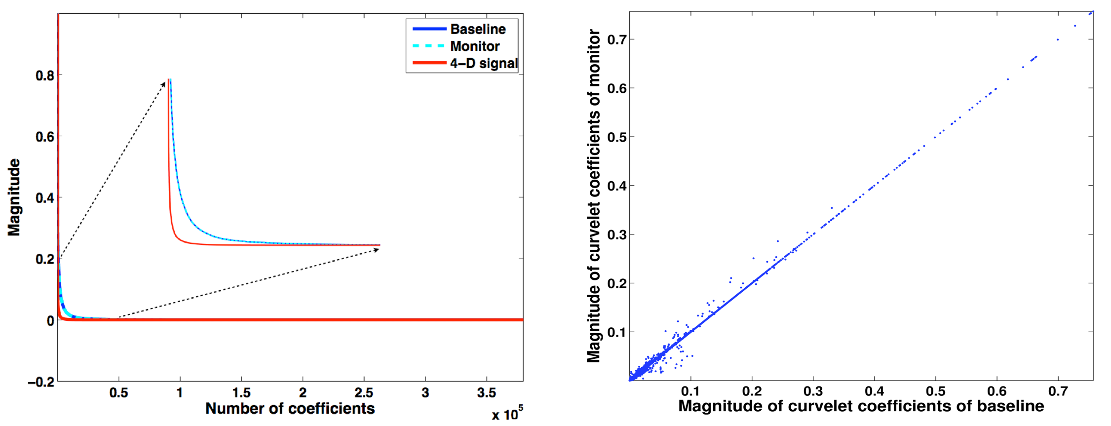
Aside from invoking randomizations during subsampling, CS exploits structure residing within seismic data volumes during reconstruction—the better the compression the better the reconstruction becomes for a given set of measurements. If we consider the surveys separately, curvelets are good candidates to reveal this structure because they concentrate the signal’s energy into few large-magnitude coefficients and many small coefficients (see left-hand side plot in Figure 1). Curvelets have this ability because they decompose seismic data into multiscale and multi-angular localized waveforms. As the cross plot in Figure 1 reveals (right-hand side plot), the curvelet transform’s ability to compress seismic data and time-lapse difference (left-hand side plot Figure 1) is not the only type of structure that we can exploit. The fact that most of the magnitudes of the curvelet coefficients of two common-receiver gathers from a 2-D OBS time-lapse survey (see Figure 8) nearly coincide indicate that the data from the two vintages shares lots of information in the curvelet domain. Therefore, we can further exploit this complementary structure during time-lapse recovery from randomized subsampling in order to improve the repeatability.
Joint recovery method (JRM)
Baron et al. (2009) introduced and analyzed mathematically a model for distributed CS where jointly sparse signals are recovered jointly. Aside from permitting sparse representations individually, jointly sparse signals share information. For instance, sensor arrays aimed at the same object tend to share information (see Xiong et al. (2004) and the references therein) and time-lapse seismic surveys are no exception.
There are different ways to incorporate this shared information amongst the different vintages. We found that we get the best recovery result if we exploit the common component amongst the baseline and monitor data explicitly. This means that for two-vintage surveys we end up with three unknown vectors. One for the common component, denoted by \(\vector{z}_0\), and two for the innovations \(\vector{z}_j\) for \(j\in {1,2}\) with respect to this common component that is shared by the vintages. In this model, the vectors for the vintages are given by \[ \begin{equation} \vector{x}_j = \vector{z}_0 + \vector{z}_j, \qquad j \in {1,2}. \label{eqjrm} \end{equation} \] As we can see, the vintages contain the common component \(\vector{z}_0\) and the time-lapse difference is contained within the difference between the innovations \(\vector{z}_j\) for \(j\in {1,2}\). Because \(\vector{z}_0\) is part of both surveys, the observed measurements are now given by \[ \begin{equation} \begin{aligned} \begin{bmatrix} \vector{y}_1\\ \vector{y}_2\end{bmatrix} &= \begin{bmatrix} {\vector{A}_1} & \vector{A}_{1} & \vector{0} \\ {\vector{A}_{2} }& \vector{0} & \vector{A}_{2} \end{bmatrix}\begin{bmatrix} \vector{z}_0 \\ \vector{z}_1 \\ \vector{z}_2 \end{bmatrix},\quad\text{or} \\ \vector{y} &= \vector{A}\vector{z}. \end{aligned} \label{jrmobs} \end{equation} \] In this expression, we overloaded the symbol \(\vector{A}\), which from now on refers to the matrix linking the observations of the time-lapse surveys to the common component and innovations pertaining to the different vintages. The above joint recovery model readily extends to \(J>2\) surveys, yielding a \(J\times \, (\text{number of vintages}+1)\) system.
Contrary to the IRS, which essentially corresponds to setting the common component to zero so there is no communication between the different surveys, both vintages share the common component in Equation \(\ref{jrmobs}\). As a result correlations amongst the vintages will be exploited if we solve instead \[ \begin{equation} \widetilde{\vector{z}}= \argmin_{\vector{z}}\|\vector{z}\|_1 \quad \text{subject to} \quad \vector{y} = \vector{Az}. \label{eqjrm2} \end{equation} \] As a result, we seek solutions for the common component and innovations that have the smallest \(\ell_1\)-norm such that the observations explain both the incomplete recordings for both vintages. Estimates for the finely sampled vintages are readily obtained via Equation \(\ref{eqjrm}\) with the recovered \(\widetilde{\vector{z}}\) while the time-lapse difference is computed via \(\widetilde{\vector{z}}_1-\widetilde{\vector{z}}_2\).
Albeit recent progress has been made (X. Li, 2015), precise recovery conditions for JRM are not yet very well studied. Moreover, the JRM was also not designed to compute differences between the innovations. To gain some insight on our formulation, we will first compare the performance of IRS and JRM in cases where the surveys are exactly replicated (\(\vector{A}_1=\vector{A}_2\)), partially replicated (\(\vector{A}_1\) and \(\vector{A}_2\) share certain fractions of rows), or where \(\vector{A}_1\) and \(\vector{A}_2\) are statistically completely independent. To get reliable statistics on the recovery performance for the different recovery schemes, we repeat a series of small stylized problems thousands of times. These small stylized examples serve as proxies for seismic acquisition problems that we will discuss later.
Stylized experiments
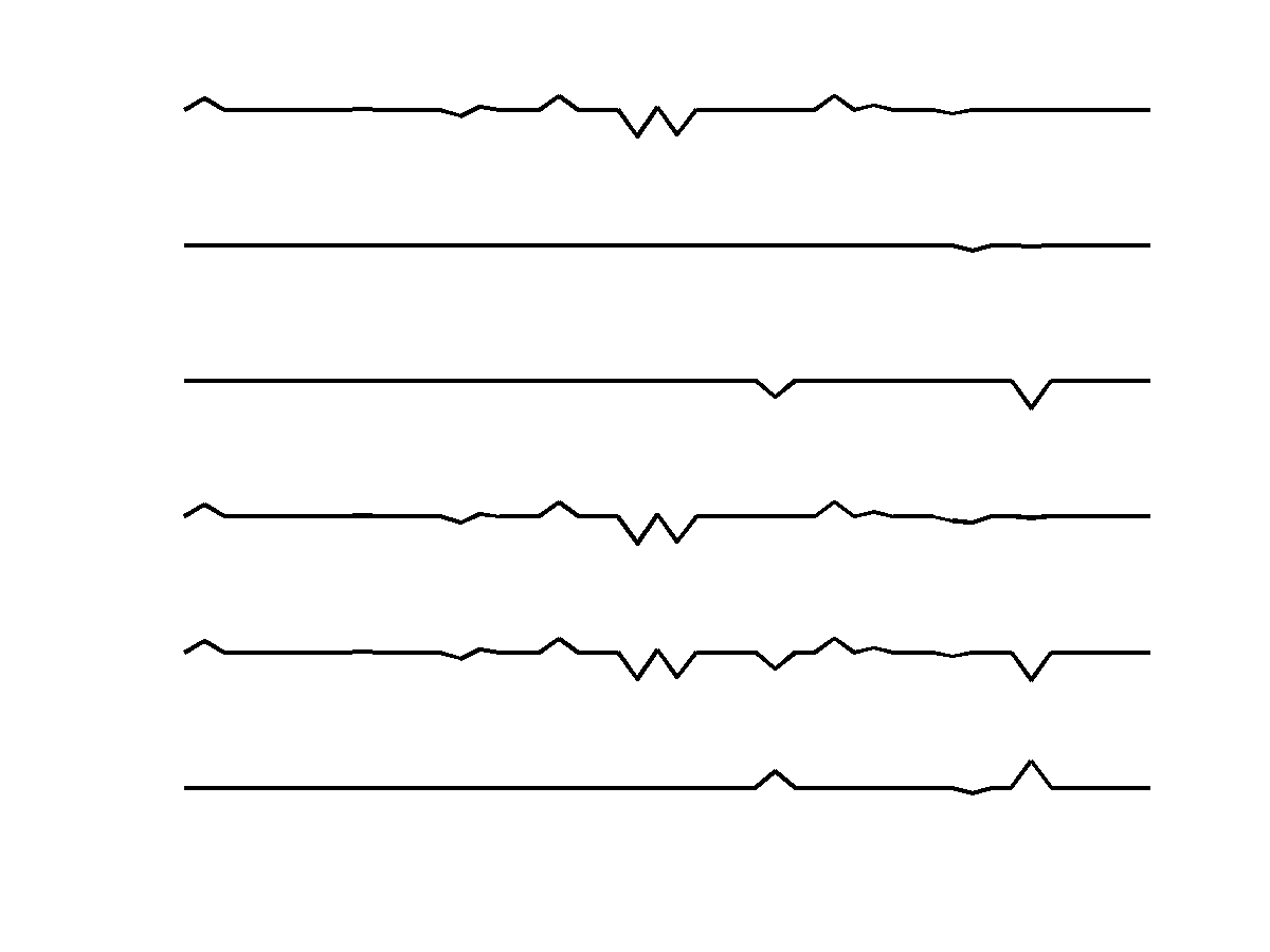
To collect statistics on the performance of the different recovery strategies, we repeat several series of small experiments many times. Each random time-lapse realization is represented by a vector with \(N = 50\) elements that has \(k=13\) nonzero entries with Gaussian distributed weights that are located at random locations such that the number of nonzero entries in each innovation is two—i.e., \(k_1 = k_2 = 2\). This leaves \(11\) nonzeros for the common component. For each random experiment, \(n=\{10,11, \cdots, 40\}\) observations \(\vector{y}_1\) and \(\vector{y}_2\) are collected using Equation \(\ref{eqSamp}\) for Gaussian matrices \(\vector{A}_1\) and \(\vector{A}_2\) that are redrawn for each repeated experiment. These Gaussian matrices have independent identically distributed Gaussian entries and serve as a proxy for randomized acquisitions in the field. An example of the time lapse vectors \(\vector{z}_0,\vector{z}_1,\vector{z}_2,\vector{x}_1,\vector{x}_2\), and \(\vector{x}_1-\vector{x}_2\) involved in these experiments is included in Figure 2. Our goal is to recover estimates for the vintages and time-lapse signals—i.e., we want to obtain the estimates \(\evector{x}_1\) and \(\evector{x}_2\), and their difference \(\evector{x}_1 - \evector{x}_2\) from subsampled measurements \(\vector{y}_1\) and \(\vector{y}_2\). When using the joint recovery model, we compute estimates for the jointly sparse vectors via \(\evector{x}_1 = \evector{z}_0 + \evector{z}_1\), and \(\evector{x}_2 = \evector{z}_0 + \evector{z}_2\), where \(\evector{z}\) is found by solving Equation \(\ref{eqjrm2}\).
To get reliable statistics on the probability of recovering the vectors representing the vintages and the time-lapse differences, we choose to perform \(M = 2000\) repeated time-lapse experiments generating \(M\) different realizations for \(\vector{y}_1\) and \(\vector{y}_2\) from different realizations of \(\vector{x}_1\) and \(\vector{x}_2\). Next, we recover \(\evector{x}_1\) and \(\evector{x}_2\) from these measurements using the IRS or JRM. From these estimates, we compute empirical probabilities of successful recovery via \[ \begin{equation} P(\vector{x}) = \dfrac{\text{Number of times} \dfrac{\|\vector{x}-\tilde{\vector{x}}\|_2}{\|\vector{x}\|_2} < \rho}{M }. \label{eqProb} \end{equation} \] We set the relative error threshold to \(\rho = 0.1\). The vector \(\vector{x}\) either represents the vintages or the difference. In case of the vintages, we multiply the probabilities.
Experiment 1—independent versus joint recovery
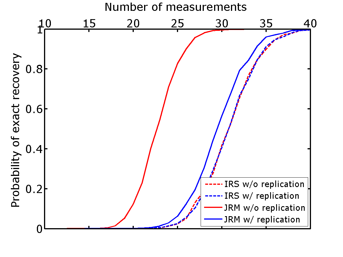
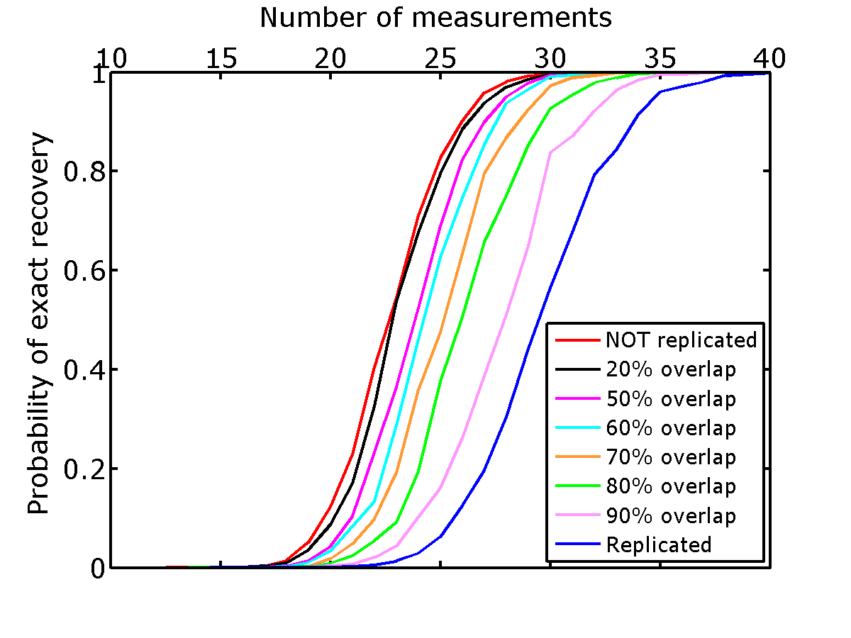
To reflect current practices in time-lapse acquisition—where people aim to replicate the surveys—we run the experiments by drawing the same random Gaussian matrices of size \(n \times N\) for \(n=\{10,11, \cdots, 40\}\) and \(N=50\) for \(\vector{A}_1\) and \(\vector{A}_2\)—i.e., \(\vector{A}_1 = \vector{A}_2\). We conduct the same experiments where the surveys are not replicated by drawing statistically independent measurement matrices for each repeated experiment, yielding \(\vector{A}_1 \neq \vector{A}_2\). For each series of experiments, we recover estimates \(\evector{x}_1\), \(\evector{x}_2\), and \(\evector{x}_1-\evector{x}_2\) from which we compute the corresponding recovery probabilities using Equation \(\ref{eqProb}\). The results are plotted in Figure 3 for the recovery of the vintages (Figure 3a) and time-lapse difference (Figure 3b).
The results of these experiments indicate that regardless of the number of measurements, JRM leads to improved recovery compared to IRS because it exploits information shared by the two jointly sparse vectors representing the vintages. The recovery probabilities for JRM (solid lines in Figure 3) show an overall improvement for both the time-lapse vectors and the time-lapse difference vector—all probability curves are to the left compared to those from IRS meaning that recovery is more likely for fewer measurements. For the time-lapse vectors, this improvement is much more pronounced for measurement matrices that are statistically independent—i.e., not replicated (\(\vector{A}_1 \neq \vector{A}_2\)). This observation is consistent with distributed compressive sensing, which predicts significant improvements when the time-lapse vectors share a significant common component. In that case, the shared component benefits most from being observed by both surveys (via the first column of \(\vector{A}\), cf. Equation \(\ref{jrmobs}\)). The IRS results for the time-lapse vectors are much less affected whether the survey is replicated or not, which makes sense because the processing is done in parallel and independently. This suggests that for time-lapse seismic, independent surveys give additional information on the sparse structure of the vintages that is reflected in their improved recovery quality. Another likely interpretation is that time-lapse data obtained via JRM has better repeatability compared to data obtained via IRS.
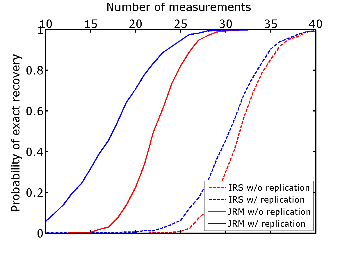
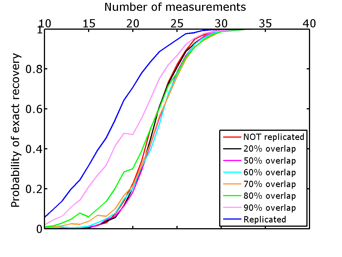
While independent surveys improve recovery with JRM, the recovery probability of the time-lapse difference vectors improves drastically when the experiments are replicated exactly. The reason for this is that the JRM simplifies to the recovery of the time-lapse differences alone in cases where the time-lapse measurements are exactly replicated. Since these time-lapse differences are sparser than the vintage vectors themselves, the time-lapse difference vectors are well recovered while the time-lapse vectors themselves are not. This result is not surprising since the error in reconstructing the vintages cancels out in the difference. This means that in CS, if one is interested in the time-lapse difference, exact repetition of the survey is preferred. However, this approach does not provide any additional structural information in the vintages. We will revisit this observation in Experiment 2 to see how the recovery performs when we have varying degrees of repeatability in the measurements.
Experiment 2—impact of degree of survey replicability
So far, we explored only two extremes, namely recovery of vintages with absolutely no replication (\(\vector{A}_1 \neq \vector{A}_2\) and statistically independent) or exact replication (\(\vector{A}_1 = \vector{A}_2\)). To get a better understanding of how replication factors into the recovery, we repeat the experiments where we vary the degree of dependence between the surveys by changing the number of rows the matrices \(\vector{A}_1\) and \(\vector{A}_2\) have in common. When all rows are in common, the survey is replicated and the percentage of overlap between the surveys is a measure for the degree of replicability of the surveys. Since JRM clearly outperformed IRS, we only consider recovery with JRM.
As before we compute recovery probabilities from \(M = 2000\) repeated time-lapse experiments generating \(M\) different realizations for the observations. We summarize the recovery probability curves for varying degrees of overlap in Figure 4. These curves confirm that the recovery of the time-lapse vectors improves when the surveys are not replicated. As soon as the surveys are no longer replicated, the recovery probabilities for the time-lapse vectors improve. These improvements become less prominent when large percentages do not overlap and as expected reaches its maximum when the surveys become independent. Recovery of the time-lapse differences on the other hand suffers drastically when the surveys are no longer \(100\%\) replicated. When less then \(80\%\) of the surveys are no longer replicated, the recovery probabilities no longer benefit from replicating the surveys. Recovery of the time-lapse vectors, on the other hand, already improves significantly at this point.
While these experiments are perhaps too idealized and small to serve as a strict guidance on how to design time-lapse surveys, they lead to the following observations. Firstly, the recovery probabilities improve when we exploit joint sparsity amongst the time-lapse vectors via JRM. Secondly, since the joint component is observed by all surveys recovery of the common component and therefore vintages improves if the surveys are not replicated. Thirdly, the time-lapse differences benefit from high degrees of replication of the surveys. In that case, the JRM degenerates to recovery of the time-lapse difference alone and as a consequence the time-lapse vectors are not well recovered.
Even though the quality of the time-lapse difference is often considered as a good means of quality control, we caution the reader to draw the conclusion that we should aim to replicate the surveys. The reason for this is that time-lapse differences are generally computed from poststack attributes computed from finely sampled, and therefore recovered, prestack baseline and monitor data and not from prestack differences. Therefore, recovery of time-lapse difference alone may not be sufficient to draw firm conclusions. Our observations were also based on very small idealized experiments that did not involve stacking and permit exact replication, which may not be realistic in practice.
Experimental setup—on-the-grid time-lapse randomized subsampling
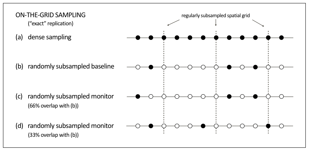
One of the main parts of the experimental setup for the synthetic seismic case study is how we define the underlying grid on which samples are taken. In context of this paper, we assume that the samples are taken on a discrete grid—i.e., samples lie “exactly” on the grid. It is also important to note that we randomly subsample the grid. As mentioned in the compressive sensing section above, randomized subsampling introduces incoherent subsampling related artifacts that are removed during sparsity-promoting signal recovery. Figure 5 shows a schematic comparison between different random realizations of a subsampled grid. As illustrated in the schematic, random samples are taken exactly on the grid. We define the term “overlap” as the percentage of on-the-grid shot locations exactly replicated between two (or more) time-lapse surveys. For the synthetic seismic case study, whenever there is an overlap between the surveys (e.g., \(50\%\), \(33\%\), \(25\%\), etc.) the on-the-grid shot locations are exactly replicated for the baseline and monitor surveys. Similarly, for the stylized experiments, when two rows of the Gaussian matrices are the same it can be interpreted as if we hit the same shot location for both the baseline and monitor surveys. Therefore, we either assume that the experimental circumstances are ideal or alternatively we can think of this assumption as ignoring the effects of being off the grid. The companion paper analyses the effects of the more realistic off-the-grid sampling. In summary, we consider the case where measurements are exactly replicated whenever we choose to visit the same shot location for the two surveys. However, because we are subsampled we need not choose to revisit all the shot locations of the baseline survey.
Synthetic seismic case study—time-lapse marine acquisition via time-jittered sources
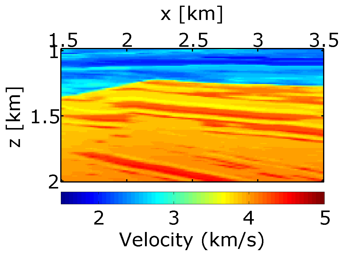
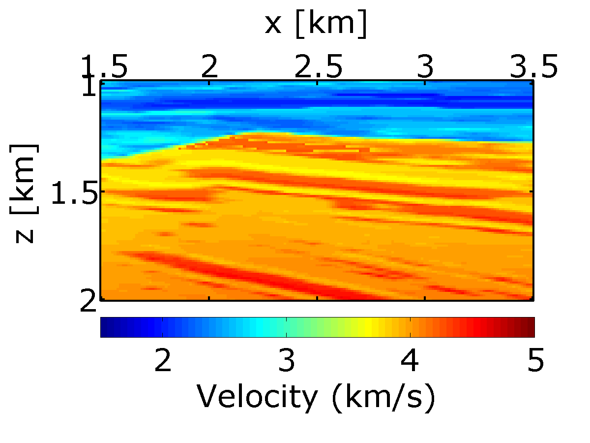
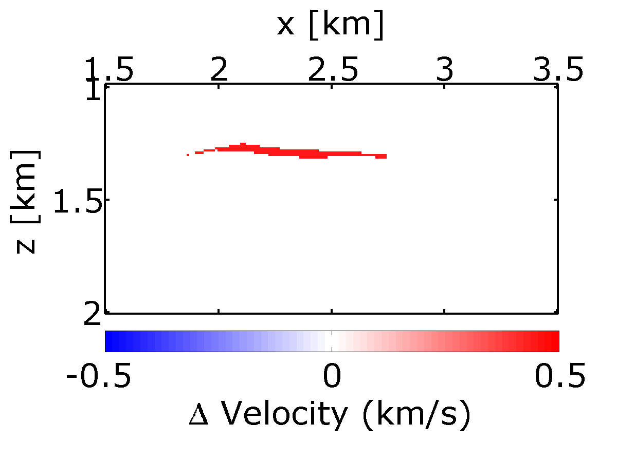
To study a more realistic example, we carry out a number of experiments on 2-D seismic lines generated from a synthetic velocity model—the BG COMPASS model (provided by BG Group). To illustrate the performance of randomized subsamplings—in particular the time-jittered marine acquisition—in time-lapse seismic, we use a subset of the BG COMPASS model (Figure 6a) for the baseline. We define the monitor model (Figure 6b) from the baseline via a fluid substitution resulting in a localized time-lapse difference at the reservoir level as shown in Figure 6c.
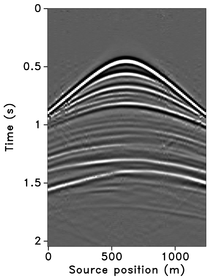
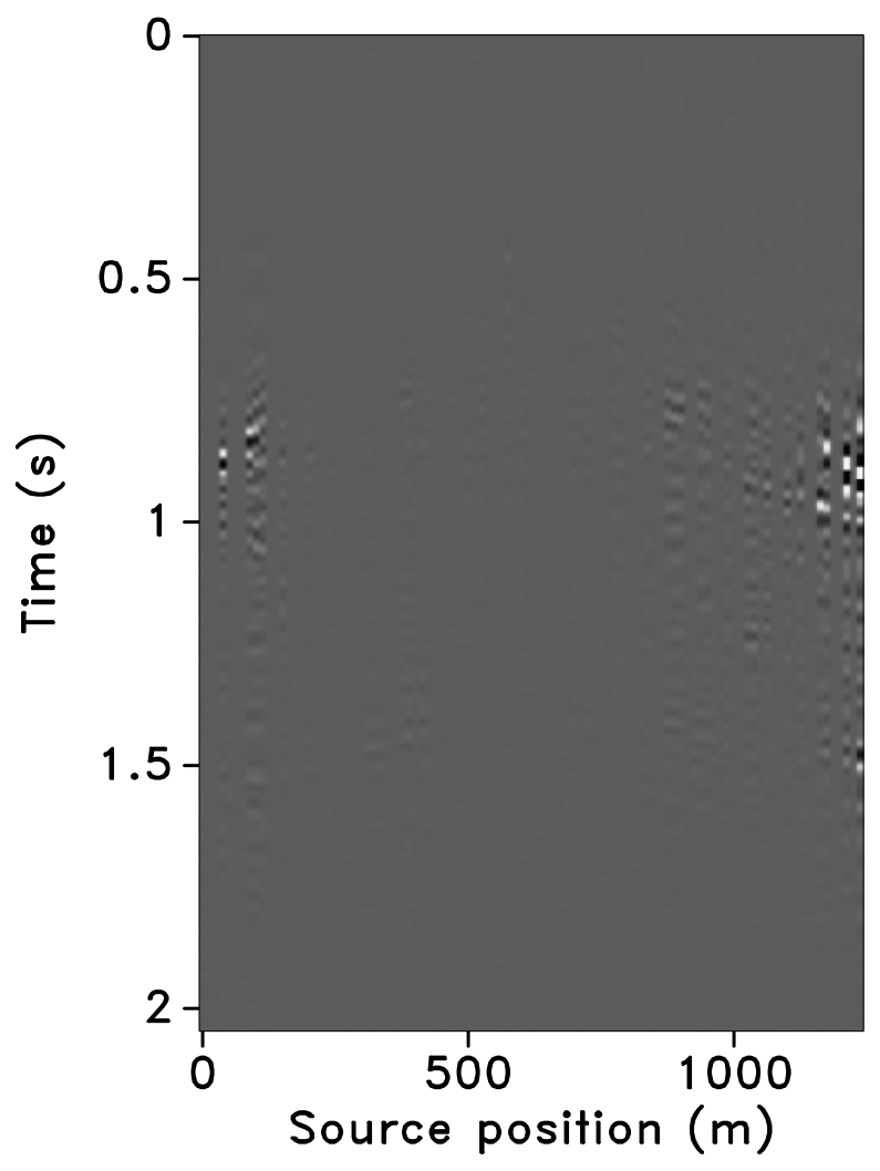
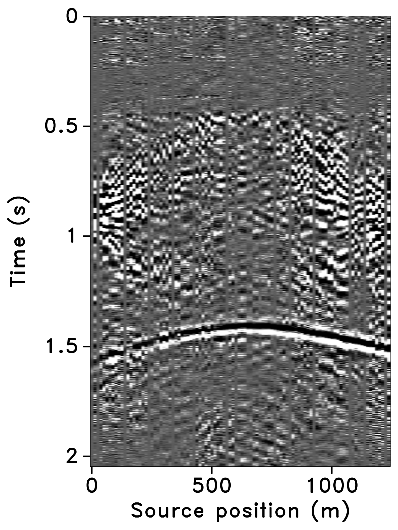
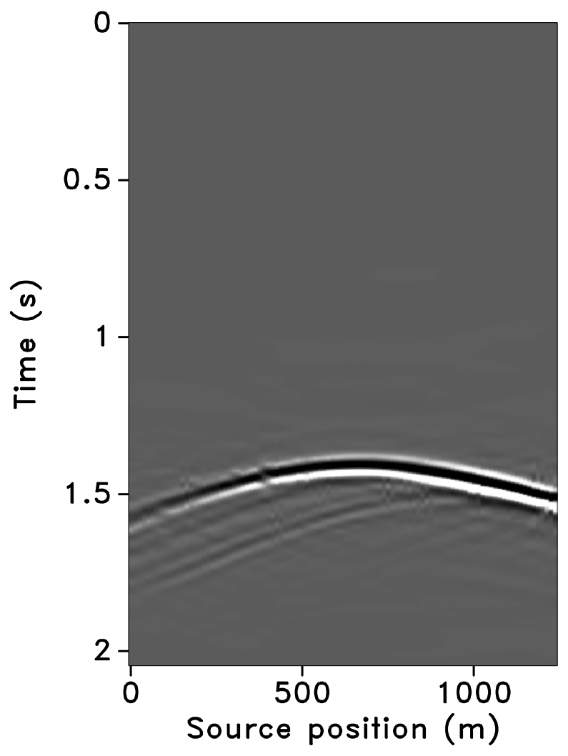
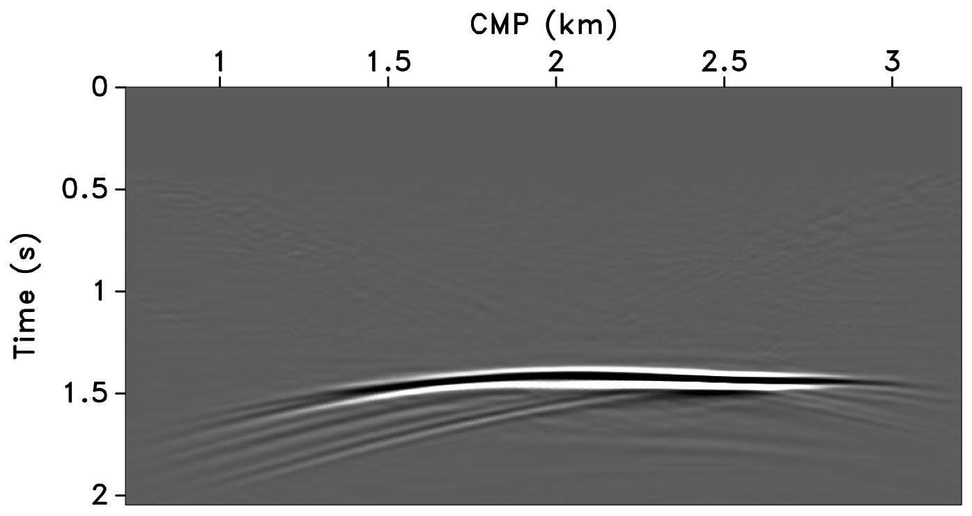
Using IWAVE (Symes, 2010) time-stepping acoustic simulation software, two acoustic datasets with a conventional source (and receiver) sampling of \(12.5\, \mathrm{m}\) are generated, one from the baseline model and the other from the monitor model. Each dataset has \(N_t = 512\) time samples, \(N_r = 100\) receivers, and \(N_s = 100\) sources. Subtracting the two datasets yields the time-lapse difference, whose amplitude is small in comparison to the two datasets (about one-tenth). Since no noise is added to the data, the time-lapse difference is simply the time-lapse signal. A receiver gather from the simulated baseline data, the monitor data and the corresponding time-lapse difference is shown in Figure 7. In order to make the time-lapse difference visible, the color axis for the figures showing the time-lapse difference is one-tenth the scale of the color axis for the figures showing the baseline and the monitor data. This colormap applies for the remainder of the paper. Also, the first source position in the receiver gathers—labeled as \(0\, \mathrm{m}\) in the figures—corresponds to \(725\, \mathrm{m}\) in the synthetic velocity model.


Time-jittered marine acquisition
Wason and Herrmann (2013) presented a pragmatic single vessel, albeit easily extendable to multiple vessels, simultaneous marine acquisition scheme that leverages CS by invoking randomness in the acquisition via random jittering of the source firing times. As a result, source interferences become incoherent in common-receiver gathers creating a favorable condition for separating the simultaneous data into conventional nonsimultaneous data (also known as “deblending”) via curvelet-domain sparsity promotion. Like missing-trace interpolation, the randomization via jittering turns the recovery into a relatively simple “denoising” problem with control over the maximum gap size between adjacent shot locations (Hennenfent and Herrmann, 2008), which is a practical requirement of wavefield reconstruction with localized sparsifying transforms such as curvelets (Hennenfent and Herrmann, 2008). The basic idea of jittered subsampling is to regularly decimate the interpolation grid and subsequently perturb the coarse-grid sample points on the fine grid. A jittering parameter, dictated by the type of acquisition and parameters such as the minimum distance (or minimum recharge time for the airguns) required between adjacent shots, relates to how close and how far the jittered sampling point can be from the regular coarse grid, effectively controlling the maximum acquisition gap. Since we are still on the grid, this is a case of discrete jittering. In this paper, we limit ourselves to the discrete case but this technique can relatively easily be taken off the grid as we discuss in the companion paper.
A seismic line with \(N_s\) sources, \(N_r\) receivers, and \(N_t\) time samples can be reshaped into an \(N\) dimensional vector \(\vector{f}\), where \(N = N_s \times N_r \times N_t\). For simplicity, we assume that all sources see the same receivers, which makes our method applicable to marine acquisition with ocean-bottom cables or nodes (OBC or OBN). As stated previously, seismic data volumes permit a compressible representation \(\vector{x}\) in the curvelet domain denoted by \(\vector{S}\). Therefore, \(\vector{f} = \vector{S}^H \vector{x}\), where \(^H\) denotes the Hermitian transpose (or adjoint), which equals the inverse curvelet transform. Since curvelets are a redundant frame (an over-complete sparsifying dictionary), \(\vector{S} \in \mathbb{C}^{P \times N}\) with \(P > N\), and \(\vector{x} \in \mathbb{C}^P\).
With the inclusion of the sparsifying transform, the matrix \(\vector{A}\) can be factored into the product of a \(n \times N\) (with \(n \ll N\)) acquisition matrix \(\vector{M}\) and the synthesis matrix \(\vector{S}^H\). The design of the acquisition matrix \(\vector{M}\) is critical to the success of the recovery algorithm. From a practical point of view, it is important to note that matrix-vector products with these matrices are matrix free—i.e., these matrices are operators that define the action of the matrix on a vector. Since the marine acquisition is performed in the source-time domain, the acquisition operator \(\vector{M}\) is a combined jittered-shot selector and time-shifting operator. Note that in this framework it is also possible to randomly subsample the receivers.
Given a baseline data vector \(\vector{f}_1\) and a monitor data vector \(\vector{f}_2\), \(\vector{x}_1\) and \(\vector{x}_2\) are the corresponding sparse representations—i.e., \(\vector{f}_1 = \vector{S}^{H}\vector{x}_1\), and \(\vector{f}_2 = \vector{S}^{H}\vector{x}_2\). Given the measurements \(\vector{y}_1 = \vector{M}_1\vector{f}_1\) and \(\vector{y}_2 = \vector{M}_2\vector{f}_2\), and \(\vector{A}_1 = \vector{M}_1\vector{S}^{H}\), \(\vector{A}_2 = \vector{M}_2\vector{S}^{H}\), our aim is to recover sparse approximations \(\widetilde{\vector{f}}_1\) and \(\widetilde{\vector{f}}_2\) by solving sparse recovery problems for the scenarios (IRS and JRM) as described above from which the time-lapse signal can be computed.
Acquisition geometry
In time-jittered marine acquisition, source vessels map the survey area firing shots at jittered time-instances, which translate to jittered shot locations for a given speed of the source vessel. Conventional acquisition with one source vessel and two airgun arrays—where each airgun array fires at every alternate periodic location—is called flip-flop acquisition. If we wish to acquire \(10.0\, \mathrm{s}\)—long shot records at every \(12.5\, \mathrm{m}\), the speed of the source vessel would have to be about \(1.25\,\mathrm{m/s}\) (approximately \(2.5\) knots). Figure 8a illustrates one such conventional acquisition scheme, where each airgun array fires every \(20.0\, \mathrm{s}\) (or \(25.0\,\mathrm{m}\)) in a flip-flop manner, traveling at about \(1.25\,\mathrm{m/s}\), resulting in nonoverlapping shot records of \(10.0\,\mathrm{s}\) every \(12.5\,\mathrm{m}\). In time-jittered acquisition, Figure 8b, each airgun array fires at every \(20.0\,\mathrm{s}\) jittered time-instances, traveling at about \(2.5\,\mathrm{m/s}\) (approximately \(5.0\) knots), with the receivers (OBC) recording continuously, resulting in overlapping (or blended) shot records (Figure 9a). Since the acquisition design involves subsampling, the acquired data volume has overlapping shot records and missing shots/traces. Consequently, the jittered flip-flop acquisition might not mimic the conventional flip-flop acquisition where airgun array 1 and 2 fire one after the other—i.e., in Figures 8b and 8c, a circle (denoting array 1) may be followed by another circle instead of a star (denoting array 2). The minimum interval between the jittered times, however, is maintained at \(10.0\,\mathrm{s}\) (typical interval required for airgun recharge) and the maximum interval is \(30.0\,\mathrm{s}\). For the speed of \(2.5\,\mathrm{m/s}\), this translates to jittering a \(50.0\,\mathrm{m}\) source grid with a minimum (and maximum) interval of \(25.0\,\mathrm{m}\) (and \(75.0\,\mathrm{m}\)) between jittered shots. Both arrays fire at the \(50.0\,\mathrm{m}\) jittered grid independent of each other.
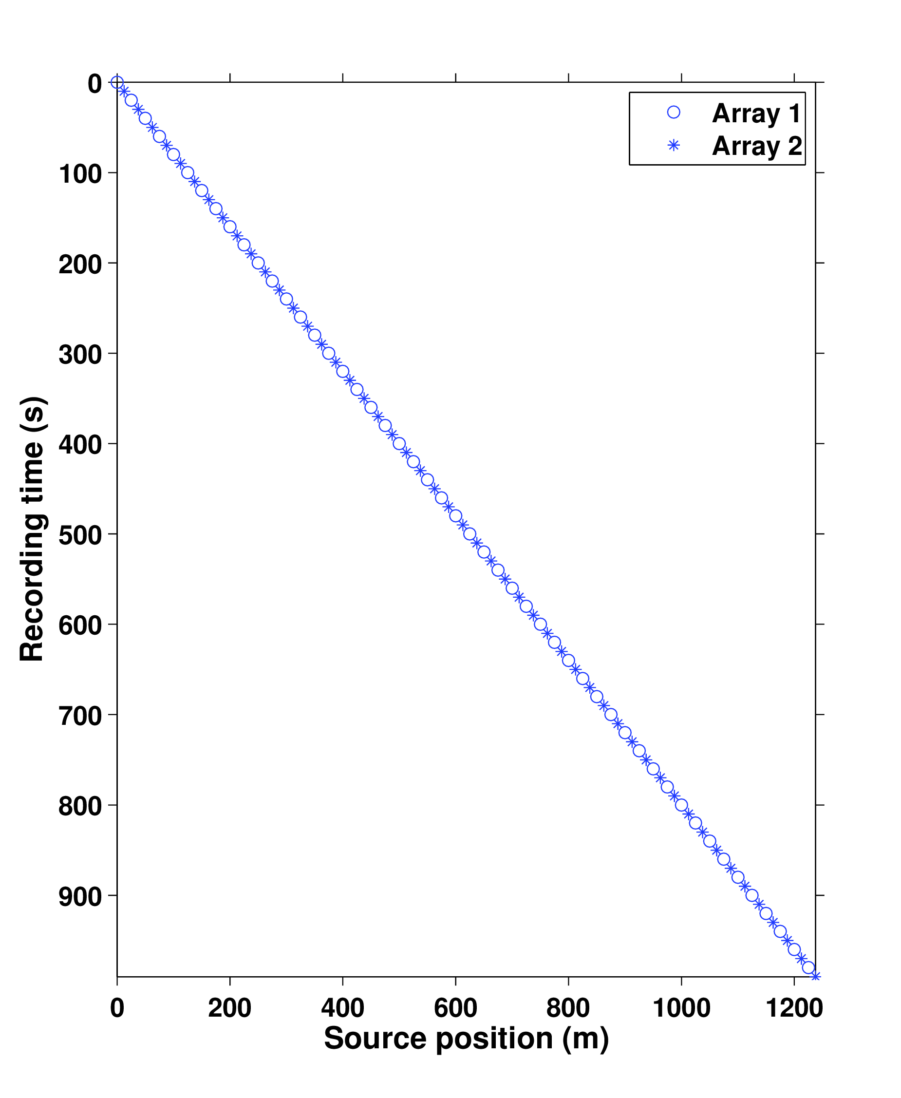
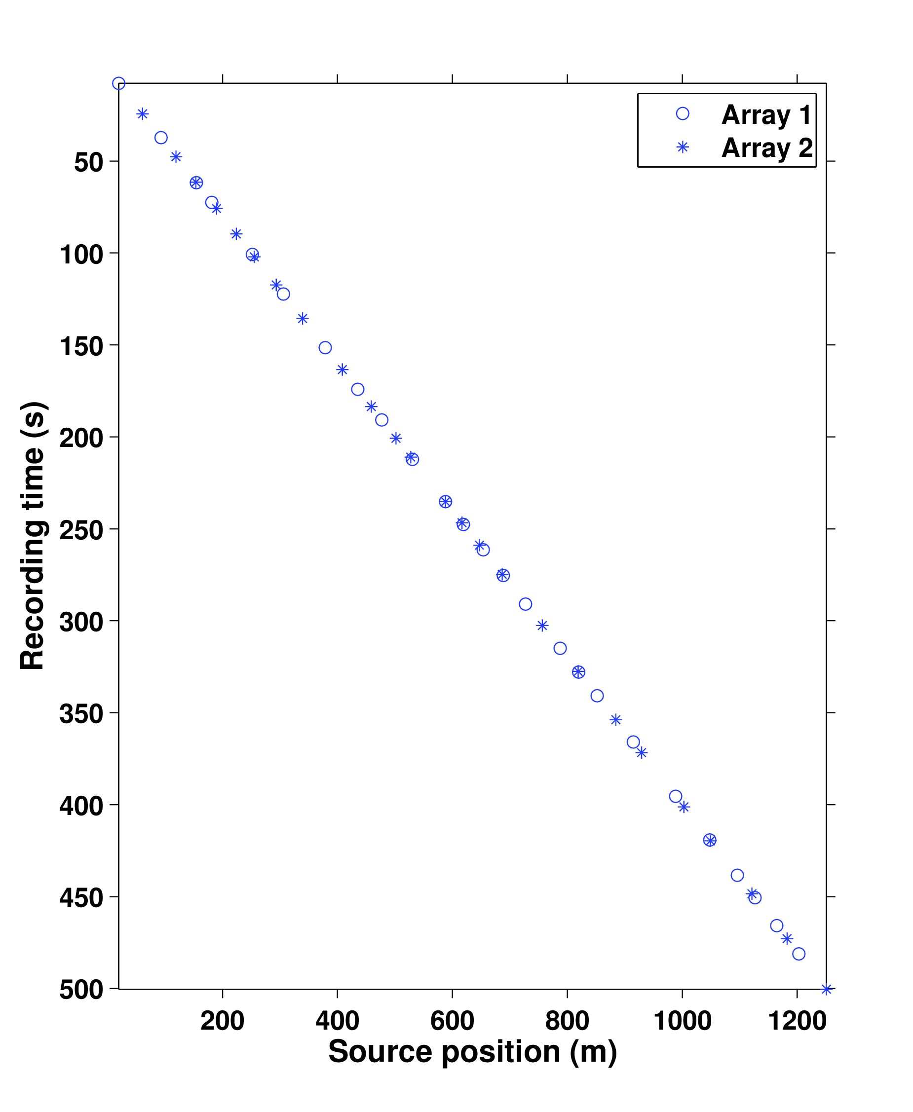
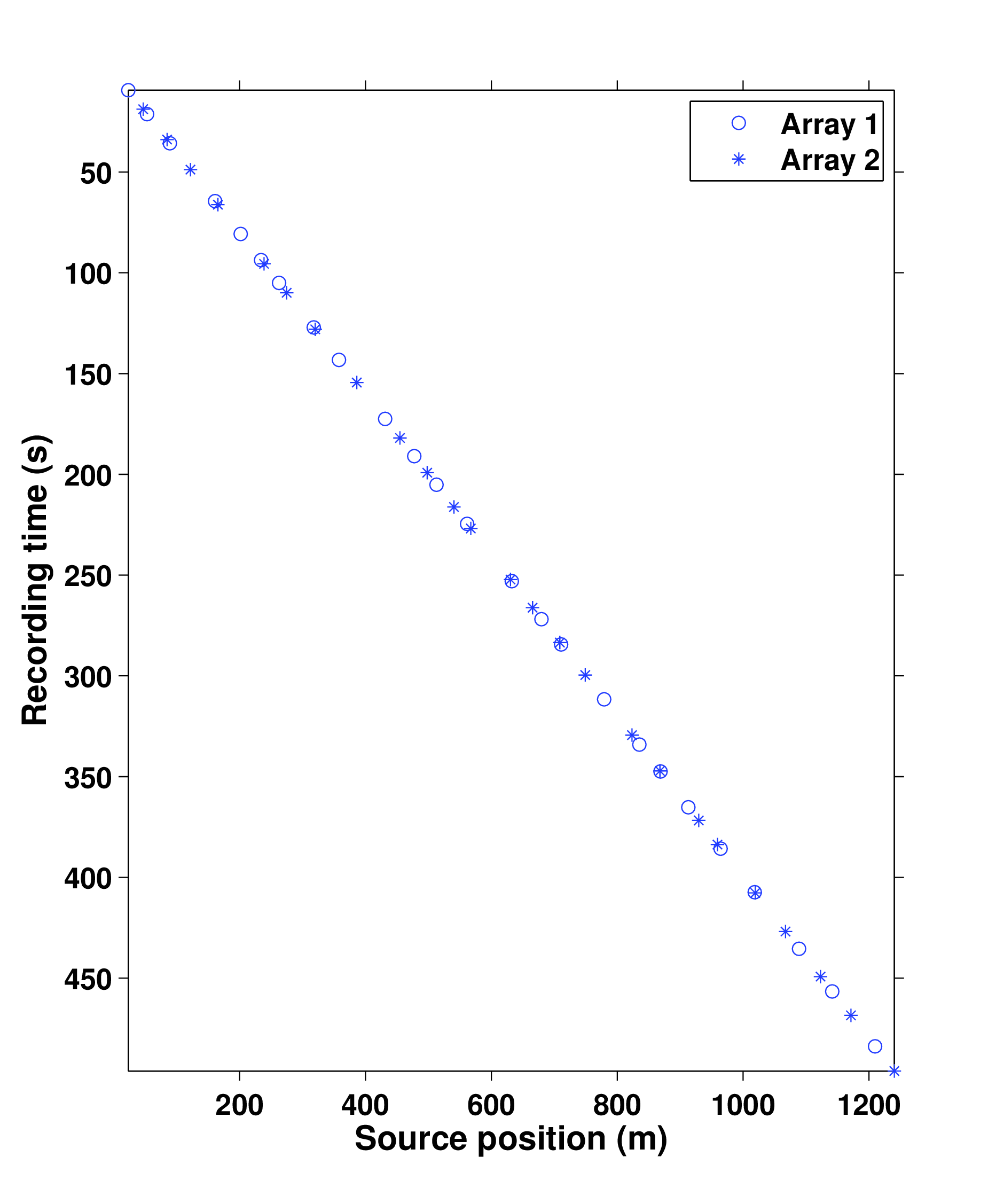
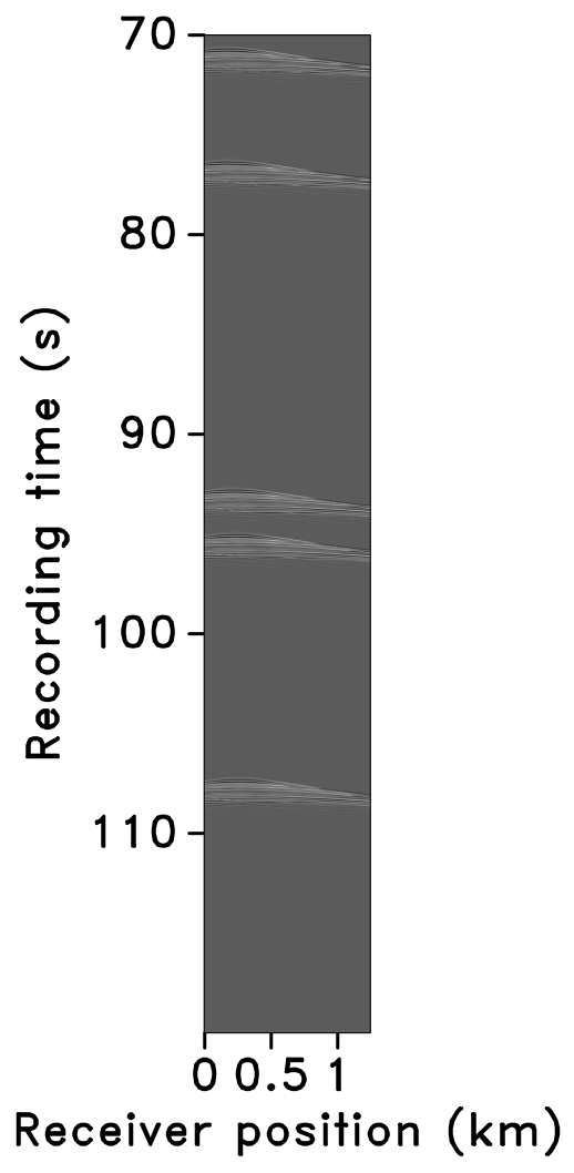
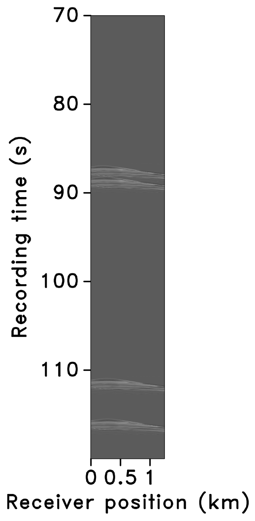
Two realizations of the time-jittered marine acquisition are shown in Figures 8b and 8c, one each for the baseline and the monitor survey. Acquisition on the \(50.0\,\mathrm{m}\) jittered grid results in an subsampling factor, \[ \begin{equation} \eta = \dfrac{1}{\text{number of airgun arrays}} \times \dfrac{\text{jittered spatial grid interval}}{\text{conventional spatial grid interval}} = \dfrac{1}{2} \times \dfrac{50.0 \text{ m}}{12.5 \text{ m}} = 2. \label{subfactor} \end{equation} \] Figures 9a and 9b show the corresponding randomly subsampled and simultaneous measurements for the baseline and monitor surveys, respectively. Note that only \(50.0\,\mathrm{s}\) of the continuously recorded data is shown. If we simply apply the adjoint of the acquisition operator to the simultaneous data—i.e., \(\vector{M}^H\vector{y}\), the interferences (or source crosstalk) due to overlaps in the shot records appear as random noise—i.e., incoherent and nonsparse, as illustrated in Figures 9c and 9d. Our aim is to recover conventional, nonoverlapping shot records from simultaneous data by working with the entire (simultaneous) data volume, and not on a shot-by-shot basis. For the present scenario, since \(\eta = 2\), the recovery problem becomes a joint deblending and interpolation problem. In contrast to conventional acquisition at a source sampling grid of \(12.5\,\mathrm{m}\) (Figure 8a), time-jittered acquisition takes half the acquisition time (Figures 8b and 8c), and the simultaneous data is separated into its individual shot records along with interpolation to the \(12.5\,\mathrm{m}\) sampling grid. The recovery problem is solved by applying the independent recovery strategy and the joint recovery method, as we will describe in the next section.


Experiments and observations
To analyze the implications of the time-jittered marine acquisition in time-lapse seismic, we follow the same sequence of experiments as conducted for the stylized examples—i.e., we compare the independent (IRS) and joint recovery methods (JRM) for varying degrees of replicability in the acquisition. Given the \(12.5 \,\mathrm{m}\) spatial sampling of the simulated (conventional) time-lapse data, applying the time-jittered marine acquisition scheme results in a subsampling factor, \(\eta = 2\) (Equation \(\ref{subfactor}\)). In practice, this corresponds to an improved efficiency of the acquisition with the same factor. Recent work (Mosher et al., 2014) has shown that factors of two or as high as ten in efficiency improvement are achievable in the field. With this subsampling factor, the number of measurements for each experiment is fixed—i.e., \(n = N/2\), each for \(\vector{y}_1\) and \(\vector{y}_2\) albeit other scenarios are possible.
We simulate different realizations of the time-jittered marine acquisition with \(100\%\), \(50\%\), and \(25\%\) overlap between the baseline and monitor surveys. Because we are in a discrete setting, these overlaps translate one-to-one into percentages of replicated on-the-grid shot locations for the surveys. Since \(\eta = 2\), and by virtue of the design of the blended acquisition, it is not possible to have two completely different (\(0\%\) overlap) realizations of the time-jittered acquisition. In all cases, we recover the deblended and interpolated baseline and monitor data from the blended data \(\vector{y}_1\) and \(\vector{y}_2\), respectively, using the independent recovery strategy (by solving Equation \(\ref{eqBP}\)) and the joint recovery method (by solving Equation \(\ref{eqjrm2}\)). As stated previously, the inherent time-lapse difference is computed by subtracting the recovered baseline and monitor data.
We perform \(100\) experiments for the baseline measurements, wherein each experiment has a different random realization of the measurement matrix \(\vector{A}_1\). Then, for each experiment, we fix the baseline measurement and subsequently work with different random realizations for the monitor survey, each corresponding to the \(50\%\) and the \(25\%\) overlap. The purpose of doing this is to examine the impact of degree of replicability of acquisition in time-lapse seismic. Table 1 summarizes the recovery results for the stacked sections, in terms of the signal-to-noise ratio defined as \[ \begin{equation} \text{SNR}(\vector{f}, \widetilde{\vector{f}}) = -20\log_{10}\frac{\|\vector{f} - \widetilde{\vector{f}}\|_2}{\|\vector{f}\|_2}, \label{SNR} \end{equation} \] for different overlaps between the baseline and monitor surveys—i.e., measurement matrices \(\vector{A}_1\) and \(\vector{A}_2\). Each SNR value is an average of \(100\) experiments including the standard deviation.
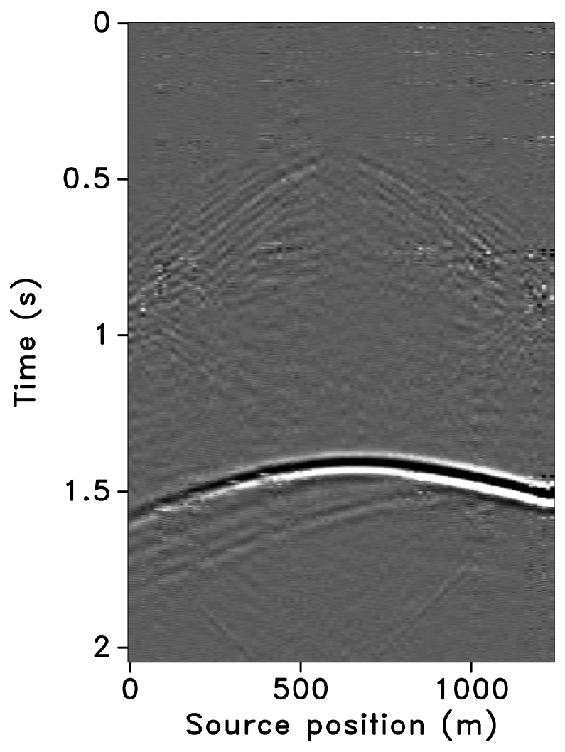
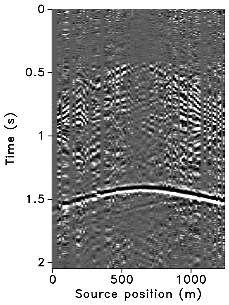
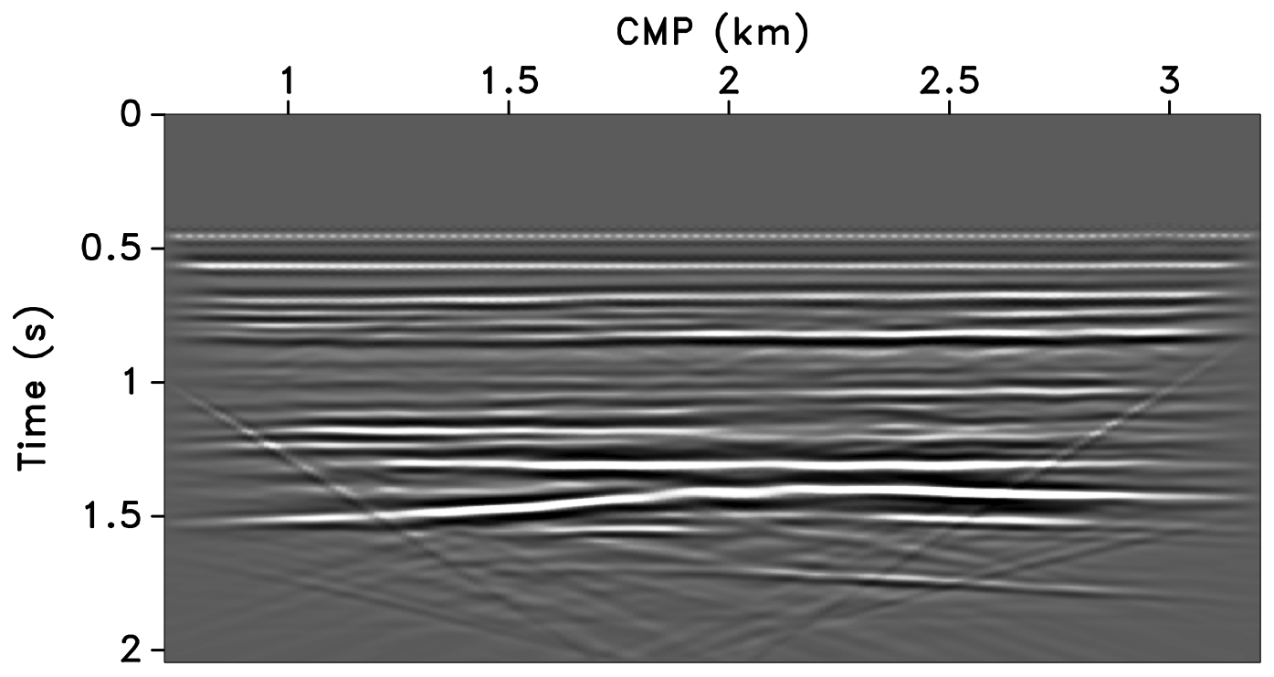
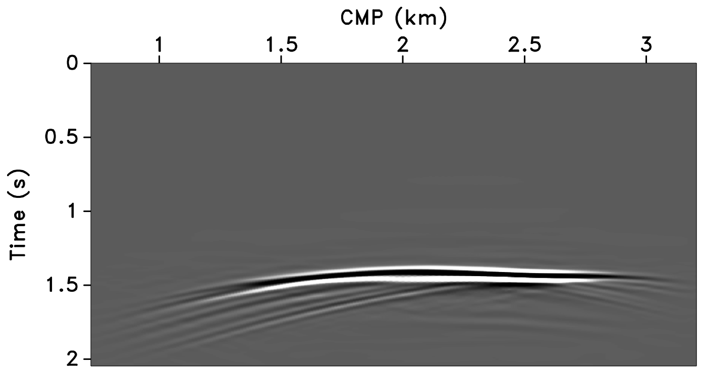
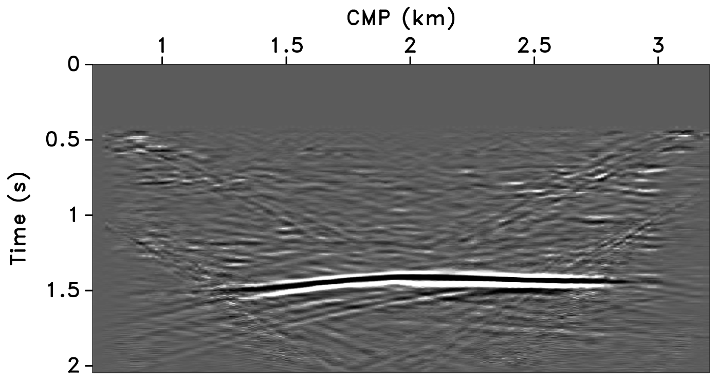
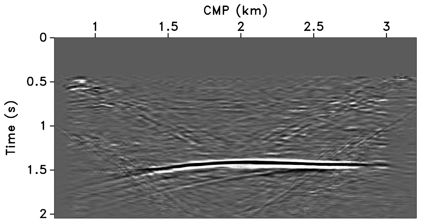
Figure 10 shows the recovered receiver gathers and difference plots for the monitor survey (for the different overlaps) using the independent recovery strategy (IRS), and Figure 11 shows the corresponding result using the joint recovery method (JRM). As illustrated in these figures, JRM leads to significantly improved recovery of the vintage compared to IRS because it exploits the shared information between the baseline and monitor data. Moreover, the recovery improves with decrease in the overlap. The IRS and JRM recovered time-lapse differences for the different overlaps are shown in Figure 12, which shows that recovery via JRM is still significantly better than IRS, however, the recovery is slightly improved with increase in the overlap. The edge artifacts in Figures 10, 11 and 12 are related to missing traces near the edges that curvelets are unable to reconstruct.
The SNRs for the stacked sections indicate a similar trend in the observations as made from the stylized experiments—i.e., (i) JRM performs better than IRS because it exploits information shared between the baseline and monitor data. Note that the SNR value, which is an average of the \(100\) experiments, for recovery of the baseline dataset via IRS is repeated for all three cases of overlap because we work with the same \(100\) realizations of the jittered acquisition throughout. However, for each of the \(100\) experiments, different realizations are drawn for the monitor survey, which explains the variations in the SNRs for the recovery via IRS. Similar fluctuations were observed by Herrmann (2010). (ii) Replication of surveys hardly affects recovery of the vintages via IRS (note similar SNRs), since the processing is done in parallel and independently. (iii) Recovery of the baseline and monitor data with JRM is better when there is a small degree of overlap between the two surveys, and it decreases with increasing degrees of overlap. As explained earlier, this behavior can be attributed to partial independence of the measurement matrices that contribute additional information via the first column of \(\vector{A}\) in Equation \(\ref{eqjrm2}\), i.e., for time-lapse seismic, independent surveys give additional structural information leading to improved recovery quality of the vintages. (iv) The converse is true for recovery of the time-lapse difference, wherein it is better if the surveys are exactly replicated. Again, as stated previously, the reason for this is the increased sparsity of the time-lapse difference itself and apparent cancelations of recovery errors due to the exactly replicated geometry.
In addition to the above observations, we find that for \(100\%\) overlap, good recovery of the stacks for IRS and JRM is possible with SNRs that are similar for the time-lapse difference and the vintages themselves. The standard deviations for the two recovery methods are also similar. One could construe that this is the ideal situation but unfortunately it is not easily attained in practice. As we move to more practical acquisition schemes where we decrease the overlap between the surveys, we see a drastic jump downwards in the SNRs for the time-lapse stack obtained with IRS. The results from JRM, on the other hand, decrease much more gradually with standard deviations that vary slightly from those for IRS, however, drops off with decrease in the overlap. In contrast, we actually see significant improvements for the SNRs of the stacks of both the baseline and monitor data with slight variations in the standard deviations.
Remember, that the number of measurements is the same for all experiments and the observed differences can be fully attributed to the performance of the recovery method in relation to the overlap between the two surveys encoded in the measurement matrices. Also, the improvements in SNRs of the vintages are significant as we lower the overlap, which goes at the expense of a relatively small loss in SNR for the time-lapse stack. However, given the context of randomized subsampling, it is important to recover the finely sampled vintages and then the time-lapse difference. In addition, time-lapse differences are often studied via differences in certain poststack attributes computed from the vintages, hence, reinforcing the importance of recovering prestack baseline and monitor data as opposed to recovering the time-lapse difference alone. While some degree of replication seemingly improves the prestack time-lapse difference, we feel that quality of the vintages themselves should prevail in the light of the above discussion. In addition, concentrating on the quality of the vintages gives us the option to compute prestack time-lapse differences in alternative ways (Wang et al., 2008).
| Overlap | Baseline | Monitor | 4-D signal | |||
|---|---|---|---|---|---|---|
| IRS | JRM | IRS | JRM | IRS | JRM | |
| \(100\%\) | 23.1 \(\pm\) 1.2 | 24.8 \(\pm\) 1.2 | 23.1 \(\pm\) 1.3 | 24.8 \(\pm\) 1.2 | 21.4 \(\pm\) 1.8 | 23.4 \(\pm\) 2.1 |
| \(50\%\) | 23.1 \(\pm\) 1.2 | 32.8 \(\pm\) 1.6 | 23.4 \(\pm\) 1.2 | 32.8 \(\pm\) 1.6 | 9.1 \(\pm\) 1.2 | 20.2 \(\pm\) 1.3 |
| \(25\%\) | 23.1 \(\pm\) 1.2 | 35.3 \(\pm\) 1.5 | 22.0 \(\pm\) 1.1 | 35.0 \(\pm\) 1.5 | 7.8 \(\pm\) 1.3 | 18.0 \(\pm\) 1.1 |
All these observations are corroborated by the plots of the recovered (monitor) receiver gathers and their differences from the original (idealized) gather in Figures 10 and 11, and the recovered time-lapse differences in Figure 12. Stacked sections of the IRS and the JRM recovered time-lapse difference are shown in Figure 13.


Repeatability measure
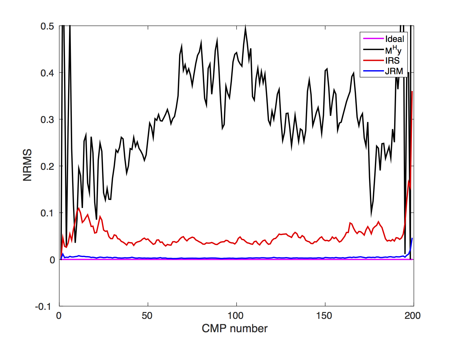
Aside from measuring SNRs, researchers have introduced repeatability measures expressing the similarity between prestack and poststack time-lapse datasets. One of the most commonly used metrics, which gives an intuitive understanding of the data repeatability, is the normalized root-mean-square (NRMS, Kragh and Christie, 2002): \[ \begin{equation} \mathrm{NRMS}=\frac{2\, \mathrm{RMS}(\tilde{\vector{f}}_2-\widetilde{\vector{f}}_1)}{\mathrm{RMS}(\widetilde{\vector{f}}_1)+\mathrm{RMS}(\widetilde{\vector{f}}_2)}, \label{NRMS} \end{equation} \] with \(\mathrm{RMS}(\widetilde{\vector{f}})\) being the root-mean-square of either vintage. This formula implies that the lower the NRMS, the higher the repeatability between the recovered datasets. Usually, lower levels of NRMS are observed for stacked data compared to prestack data since stacking reduces uncorrelated random noise. A NRMS ratio of \(0\) is achievable only in a perfectly repeatable world. In practice, NRMS ratios between \(0.2\) and \(0.3\) are considered as acceptable; ratios less than \(0.2\) are considered excellent. To further evaluate the results of our synthetic seismic experiment, we compute the NRMS ratios from stacked sections before and after recovery via IRS and JRM.
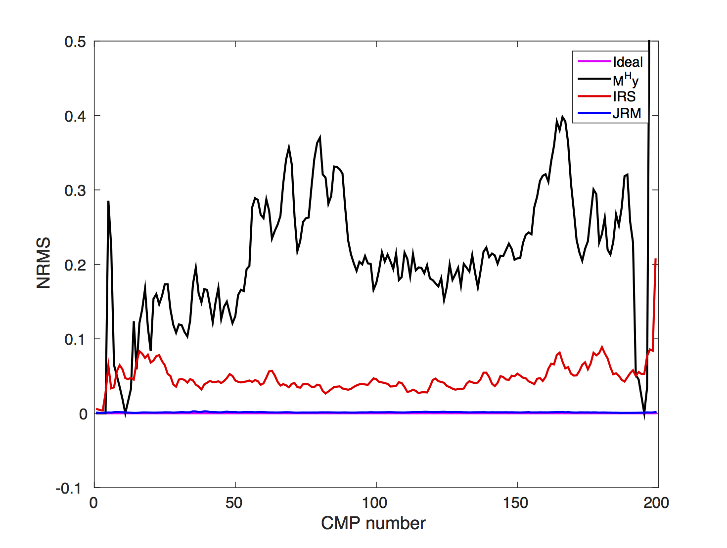
To compute this quantity, we extract time windows from stacked sections around two-way travel time between \(0.5\) s and \(1.3\, \mathrm{s}\), where we know there is no time-lapse signal present. We obtain the stacked sections before and after processing by either applying the adjoint of the sampling matrix (see discussion under Equation \(\ref{subfactor}\)) to the observed data or by solving a sparsity-promoting program. The former serves as a proxy for acquisition scenarios where one relies on the fold to stack out acquisition related artifacts. Results of this exercise for \(50\%\) overlap and \(25\%\) overlap are included in Figures 14a and 14b. These plots clearly show that (i) simply applying the adjoint, followed by stacking, leads to poor repeatability, and therefore is unsuitable for time-lapse practices; (ii) sparse recovery improves the NRMS; (iii) exploiting shared information amongst the vintages leads to near optimal values for the NMRS despite the subsampling; and finally (iv) high degrees of repeatability of recovered data are achievable from data collected with small overlaps in the acquisition geometry.
Discussion
Obtaining useful time-lapse seismic is challenging for many reasons, including cost, the need to calibrate the surveys, and the subsequent processing to extract reliable time-lapse information. Meeting these challenges in the field has resulted in acquisitions which aim to replicate the geometry of the previous survey(s) as precisely as possible. Unfortunately, this replication can be both difficult to achieve and expensive. Post acquisition, processing aims to improve the repeatability of the data such that certain (poststack) attributes can be derived reliably from the baseline and monitor surveys. Within this context, our aim is to reduce the cost and improve the quality of the prestack baseline and monitor data without relying on expensive fine sampling and high degrees of replicability of the surveys. Our methodology involves a combination of economical randomized samplings and sparsity-promoting data recovery. The latter exploits (curvelet-domain) sparsity and correlations amongst different vintages. To the authors’ knowledge, this approach is among the first to address time-lapse seismic problems in which the common component amongst vintages—and innovations with respect to this shared component—is made explicit.
The presented synthetic seismic case study, supported by the findings from the stylized examples and theoretical results from the distributed compressive sensing literature (Baron et al., 2009), represents a proof of concept for how sharing information amongst the vintages can lead to high-fidelity vintages and 4-D signals (with minor trade-offs) in a cost effective manner. This approach creates new possibilities for meeting modern survey objectives, including cost and environmental impact considerations, and improvements in spatial sampling. In this paper, even though our measurements are taken on the grid, allowing us to ignore errors related to sampling off the grid, our proposed time-lapse acquisition is low-cost since we are always subsampled in the surveys. Our joint recovery model produces finely sampled data volumes from these subsampled, and not necessarily replicable, randomized surveys. These data volumes exhibit better repeatability levels (in terms of NRMS ratios) compared to independent recovery, where correlations amongst the vintages are not exploited.
In our companion paper “Cheap time-lapse with distributed Compressive Sensing—impact on repeatability”, we demonstrate how we deal with the effects of non-replicability of the surveys when we take measurements from an irregular grid. We demonstrate that errors related to being off the grid cannot be ignored. The “bad news” is that replication is unattainable because small inevitable deviations in the shot locations amongst the time-lapse surveys negate the benefit of replication for the time-lapse signal itself. However, the good news is that a slightly deviated measurement already adds information that improves recovery of the vintages. This implies that an argument can be made to not replicate the surveys as long as we know sufficiently accurately where we fired in the field. Please remember that the claims of this paper relate to the unnecessary requirement to visit the same randomly subsampled on-the-grid shot locations during the two, or more, surveys.
Furthermore, we did not consider surveys that have been acquired in situations where there are significant variations in the water column velocities amongst the different surveys. As long as these physical changes can be modeled, we do not foresee problems. As expected using standard CS, our recovery method should be stable with respect to noise (Candès et al., 2006), but this needs to be investigated further. Moreover, recent successes in the application of compressive sensing to actual land and marine field data acquisition (see e.g. Mosher et al. (2014)) support the fact that these technical challenges with noise and calibration can be overcome in practice. Our future research will also involve working with towed-streamer surveys where other challenges like the sparse and irregular crossline sampling will be investigated.
In this study, we concentrated our efforts on producing high-quality baseline and monitor surveys from economic randomized acquisitions. There are areas of application for the joint recovery model that have not yet been explored in detail, such as imaging and full-waveform inversion problems. Early results on these applications suggest that our joint recovery model extends to sparsity-promoting imaging (Tu et al., 2011; Herrmann and Li, 2012) including imaging with surface-related multiples, and time-lapse full-waveform inversion (Oghenekohwo et al., 2015). In all applications, the use of shared information amongst vintages improves the inversion results even for acquisitions with large gaps. Finally, none of the other recently proposed approaches in this research area—e.g., double differences (Yang et al., 2014) and total-variation norm minimization on time-lapse earth models (Maharramov and Biondi, 2014)—use the shared information amongst the vintages explicitly.
Conclusions
We considered the situation of recovering time-lapse data from on-the-grid but randomly subsampled surveys. In this idealized setting, where we ignore the effects of being off the grid, we found that it is better not to revisit the on-the-grid shot locations amongst the time-lapse surveys when the vintages themselves are of prime interest. This result is a direct consequence of introducing a common component, which contains information shared amongst the vintages, as part of our proposed joint recovery method. Compared to independent recoveries of the vintages, we obtain time-lapse data exhibiting a higher degree of repeatability in terms of normalized root-mean-square ratios. Under the above stated idealized setting and ignoring complicating factors such as tidal differences, our proposed method lowers the cost and environmental imprint of acquisition because fewer shot locations are visited. It also allows us to extend the survey area or to increase the data’s resolution at the same costs as conventional surveys. Our improvements concern the vintages and not the time-lapse difference itself, which would benefit if we choose to use the same shot locations during the surveys. Because we are generally interested in “poststack” attributes derived from the vintages, their recovery took prevalence. So, we make the argument not to replicate—i.e., revisit on-the-grid shot locations during randomized surveys in cases where poststack time-lapse attributes are of interest only.
Acknowledgements
We would like to acknowledge the extraordinary contributions of one of our co-authors, Ernie Esser, especially during the preliminary composition of this paper. Ernie’s insight allowed us to have a deeper understanding of the subject matter. Unfortunately Ernie passed away in March 2015 and was not able to see this final version of the work we started together. We are also grateful to Gary Hampson for his review of our original manuscript and his insightful feedback. The authors wish to acknowledge the SENAI CIMATEC Supercomputing Center for Industrial Innovation, with support from BG Brasil and the Brazilian Authority for Oil, Gas and Biofuels (ANP), for the provision and operation of computational facilities and the commitment to invest in Research and Development. This work was financially supported in part by the Natural Sciences and Engineering Research Council of Canada Collaborative Research and Development Grant DNOISE II (CDRP J 375142-08). This research was carried out as part of the SINBAD II project with the support of the member organizations of the SINBAD Consortium.
Baron, D., Duarte, M. F., Wakin, M. B., Sarvotham, S., and Baraniuk, R. G., 2009, Distributed compressive sensing: CoRR, abs/0901.3403. Retrieved from http://arxiv.org/abs/0901.3403
Beasley, C. J., Chambers, R. E., Workman, R. L., Craft, K. L., and Meister, L. J., 1997, Repeatability of 3-d ocean-bottom cable seismic surveys: The Leading Edge, 16, 1281–1286.
Beyreuther, M., Cristall, J., and Herrmann, F. J., 2005, Computation of time-lapse differences with 3-D directional frames: SEG technical program expanded abstracts. SEG; SEG. doi:10.1190/1.2148227
Brown, G., and Paulsen, J., 2011, Improved marine 4D repeatability using an automated vessel, source and receiver positioning system: First Break, 29, 49–58.
Candes, E. J., and Tao, T., 2006, Near-optimal signal recovery from random projections: Universal encoding strategies: Information Theory, IEEE Transactions on, 52, 5406–5425.
Candès, E. J., and Wakin, M. B., 2008, An introduction to compressive sampling: Signal Processing Magazine, IEEE, 25, 21–30.
Candès, E. J., Romberg, J., and Tao, T., 2005, Signal recovery from incomplete and inaccurate measurements: Comm. Pure Appl. Math., 59, 1207–1223.
Candès, E., Romberg, J., and Tao, T., 2006, Stable signal recovery from incomplete and inaccurate measurements: Communications on Pure and Applied Mathematics, 59, 1207–1223.
Donoho, D. L., 2006, Compressed sensing: Information Theory, IEEE Transactions on, 52, 1289–1306.
Eggenberger, K., Christie, P., Manen, D.-J. van, and Vassallo, M., 2014, Multisensor streamer recording and its implications for time-lapse seismic and repeatability: The Leading Edge, 33, 150–162.
Eiken, O., Haugen, G. U., Schonewille, M., and Duijndam, A., 2003, A proven method for acquiring highly repeatable towed streamer seismic data: Geophysics, 68, 1303–1309.
Fanchi, J. R., 2001, Time-lapse seismic monitoring in reservoir management: The Leading Edge, 20, 1140–1147.
Hennenfent, G., and Herrmann, F. J., 2008, Simply denoise: Wavefield reconstruction via jittered undersampling: Geophysics, 73, V19–V28.
Herrmann, F. J., 2010, Randomized sampling and sparsity: Getting more information from fewer samples: Geophysics, 75, WB173–WB187.
Herrmann, F. J., and Hennenfent, G., 2008, Non-parametric seismic data recovery with curvelet frames: Geophysical Journal International, 173, 233–248.
Herrmann, F. J., and Li, X., 2012, Efficient least-squares imaging with sparsity promotion and compressive sensing: Geophysical Prospecting, 60, 696–712.
Herrmann, F. J., Moghaddam, P., and Stolk, C. C., 2008, Sparsity-and continuity-promoting seismic image recovery with curvelet frames: Applied and Computational Harmonic Analysis, 24, 150–173.
Koster, K., Gabriels, P., Hartung, M., Verbeek, J., Deinum, G., and Staples, R., 2000, Time-lapse seismic surveys in the north sea and their business impact: The Leading Edge, 19, 286–293.
Kragh, E., and Christie, P., 2002, Seismic repeatability, normalized rms, and predictability: The Leading Edge, 21, 640–647.
Landrø, M., 2001, Discrimination between pressure and fluid saturation changes from time-lapse seismic data: Geophysics, 66, 836–844.
Li, X., 2015, A weighted \(\ell_1\)-minimization for distributed compressive sensing: Master’s thesis,. The University of British Columbia. Retrieved from https://www.slim.eos.ubc.ca/Publications/Public/Thesis/2015/li2015THwmd/li2015THwmd.pdf
Lumley, D., 2010, 4D seismic monitoring of cO 2 sequestration: The Leading Edge, 29, 150–155.
Lumley, D. E., 2001, Time-lapse seismic reservoir monitoring: Geophysics, 66, 50–53.
Lumley, D., and Behrens, R., 1998, Practical issues of 4D seismic reservoir monitoring: What an engineer needs to know: SPE Reservoir Evaluation & Engineering, 1, 528–538.
Maharramov, M., and Biondi, B., 2014, Robust joint full-waveform inversion of time-lapse seismic data sets with total-variation regularization: ArXiv Preprint ArXiv:1408.0645.
Mansour, H., Wason, H., Lin, T. T., and Herrmann, F. J., 2012, Randomized marine acquisition with compressive sampling matrices: Geophysical Prospecting, 60, 648–662.
Mosher, C., Li, C., Morley, L., Ji, Y., Janiszewski, F., Olson, R., and Brewer, J., 2014, Increasing the efficiency of seismic data acquisition via compressive sensing: The Leading Edge, 33, 386–391.
Oghenekohwo, F., Kumar, R., Esser, E., and Herrmann, F. J., 2015, Using common information in compressive time-lapse full-waveform inversion: In 77th eAGE conference and exhibition 2015.
Porter-Hirsche, J., and Hirsche, K., 1998, Repeatability study of land data aquisition and processing for time lapse seismic:.
Rickett, J., and Lumley, D., 2001, Cross-equalization data processing for time-lapse seismic reservoir monitoring: A case study from the gulf of mexico: Geophysics, 66, 1015–1025.
Ross, C. P., and Altan, M. S., 1997, Time-lapse seismic monitoring: Some shortcomings in nonuniform processing: The Leading Edge, 16, 931–937.
Schonewille, M., Klaedtke, A., Vigner, A., Brittan, J., and Martin, T., 2009, Seismic data regularization with the anti-alias anti-leakage fourier transform: First Break, 27.
Spetzler, J., and Kvam, Ø., 2006, Discrimination between phase and amplitude attributes in time-lapse seismic streamer data: Geophysics, 71, O9–O19.
Symes, W. W., 2010, IWAVE: A framework for wave simulation:. Retrieved from http://www.trip.caam.rice.edu/software/iwave/doc/html/
Tegtmeier-Last, S., and Hennenfent, G., 2013, System and method for processing 4d seismic data:. Google Patents.
Tu, N., Lin, T. T., and Herrmann, F. J., 2011, Sparsity-promoting migration with surface-related multiples: EAGE. EAGE; EAGE. Retrieved from https://www.slim.eos.ubc.ca/Publications/Public/Conferences/EAGE/2011/tu11EAGEspmsrm/tu11EAGEspmsrm.pdf
Van Den Berg, E., and Friedlander, M. P., 2008, Probing the pareto frontier for basis pursuit solutions: SIAM Journal on Scientific Computing, 31, 890–912.
Wang, D., Saab, R., Yilmaz, Ö., and Herrmann, F. J., 2008, Bayesian wavefield separation by transform-domain sparsity promotion: Geophysics, 73, A33–A38.
Wason, H., and Herrmann, F. J., 2013, Time-jittered ocean bottom seismic acquisition: SEG technical program expanded abstracts. doi:10.1190/segam2013-1391.1
Wason, H., Oghenekohwo, F., and Herrmann, F. J., 2015, Compressed sensing in 4-D marine-recovery of dense time-lapse data from subsampled data without repetition: EAGE annual conference proceedings. UBC; UBC. doi:10.3997/2214-4609.201413088
Xiong, Z., Liveris, A. D., and Cheng, S., 2004, Distributed source coding for sensor networks: Signal Processing Magazine, IEEE, 21, 80–94.
Xu, S., Zhang, Y., Pham, D., and Lambaré, G., 2005, Antileakage fourier transform for seismic data regularization: Geophysics, 70, V87–V95.
Yang, D., Malcolm, A., and Fehler, M., 2014, Time-lapse full waveform inversion and uncertainty analysis with different survey geometries: In 76th eAGE conference and exhibition 2014.