Simply denoise: wavefield reconstruction via jittered undersampling

Synthetic data example

Figure 7(a) shows a synthetic dataset sampled above Nyquist rate along both the time and receiver axes. The corresponding amplitude spectrum is plotted in Figure 7(b). These two figures serve as references. Comparisons are made between the interpolation results of three-fold spatially undersampled data, collected either regularly or optimally-jittered. As expected, the amplitude spectrum (Figure 8(c)) of the regularly undersampled data (Figure 8(a)) is severely aliased. Unfortunately, these coherent $f$ -$k$ undersampling artifacts remain coherent in the curvelet domain and hence create a challenge for the reconstruction. To the contrary, there is no observable coherent spectral leakage in the amplitude spectrum (Figure 8(d)) for the optimally-jittered undersampled data (Figure 8(b)). Instead, the amplitude spectrum looks noisy in the temporal frequency band of the seismic signal.

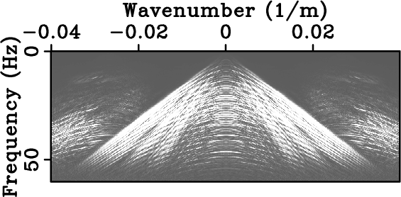
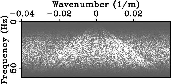
Figure 9 shows the CRSI results for these two experiments. Figures 9(a) and 9(b) depict the reconstructions given data regularly (Figure 8(a)) and optimally-jittered (Figure 8(b)) sampled, respectively. Figures 9(c) and 9(d) represent the corresponding amplitude spectra. Unlike Figure 9(d) that is only slightly corrupted by incoherent errors, Figure 9(c) still contains substantial energy from the coherent undersampling artifacts. This observation is corroborated by the respective signal-to-reconstruction-error-ratios of 6.91 dB and 10.42 dB. The signal-to-reconstruction-error-ratio, defined as $20\cdot\log_{10}(\Vert\ensuremath{\mathbf{f}}_0\Vert _2/\Vert\ensuremath{\mathbf{f}}_0-\tilde{\ensuremath{\mathbf{f}}}\Vert _2)$ , accounts for the energy of the error but not its type. It is important to keep in mind that the difference in reconstruction quality is solely due to the difference in spatial sampling, the undersampling factor and the recovery procedure were kept the same. This behavior leads us to conclude that, for a given undersampling factor, spatial optimally-jittered undersampling is (much) more favorable for CRSI than regular undersampling.

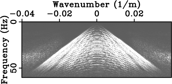
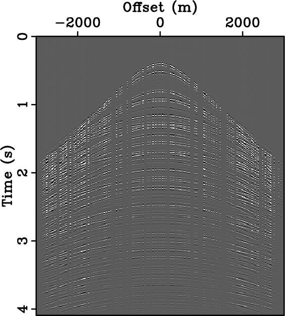
In addition, Figure 10 shows a recovery experiment given randomly three-fold spatially undersampled data. Figure 10(a) depicts the simulated acquired data and Figure 10(b) the CRSI result. The signal-to-reconstruction-error-ratio is 9.72 dB. Figures 10(c) and 10(d) contain the corresponding amplitude spectra. As can be observed by comparing Figure 8(d) with Figure 10(c), both random and optimally-jittered samplings create favorable recovery conditions. However, the larger size of the acquisition gaps in randomly undersampled data deteriorates the overall performance of CRSI. This result corroborates the importance of controlling the size of the maximum gap in optimally-jittered undersampling for reconstruction with curvelets.

data_12p5m,fkdata_12p5m
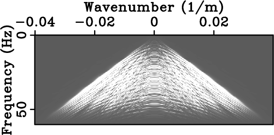
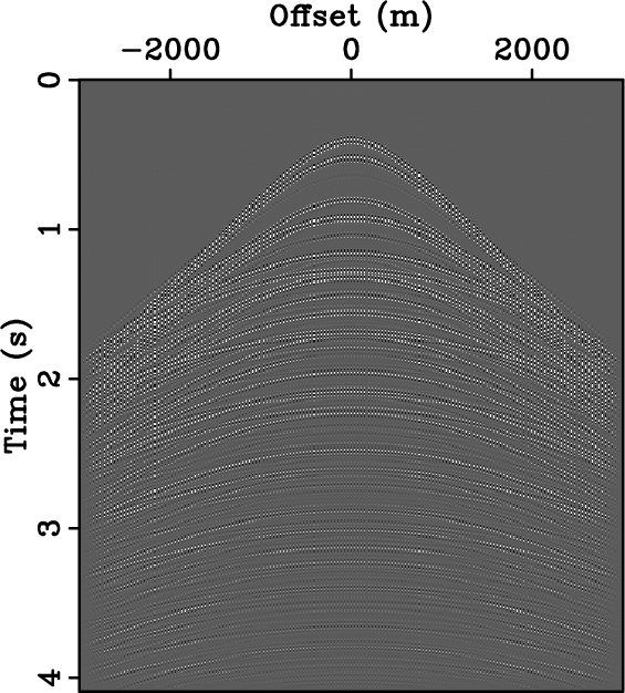
Figure 7. Reference model. (a) Synthetic data sampled above Nyquist rate and (b) corresponding amplitude spectrum.

data_subREG,data_subIRREG,fkdata_subREG,fkdata_subIRREG
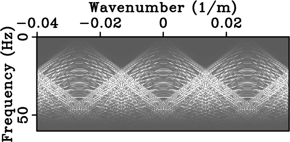
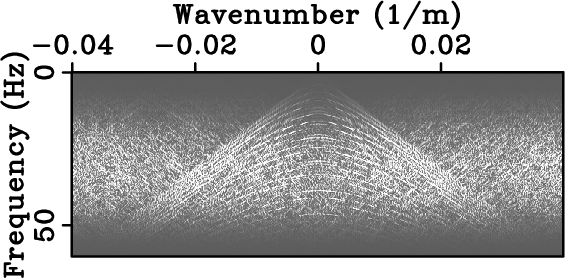
Figure 8. Synthetic data of Figure 7 (a) regularly and (b) optimally-jittered three-fold undersampled along the spatial axis. Their respective amplitude spectra are plotted in (c) and (d). For the same amount of acquired data, optimally-jittered undersampling turns the harmful coherent undersampling artifacts of regular undersampling, i.e., aliases, into incoherent random noise.

crsi_subREG,crsi_subIRREG,fkcrsi_subREG,fkcrsi_subIRREG
Figure 9. Curvelet reconstructions with sparsity-promoting inversion. Results given (a) data of Figure 8(a) and (b) data of Figure 8(b). The respective signal-to-reconstruction-error-ratios are 6.91 dB and 10.42 dB. For the same amount of data collected in the field, the reconstruction from optimally-jittered undersampled data is much more accurate than the reconstruction from regularly undersampled data.

data_subRAND,crsi_subRAND,fkdata_subRAND,fkcrsi_subRAND
Figure 10. Randomly undersampled data and curvelet reconstruction with sparsity-promoting inversion. (a) Synthetic data randomly three-fold undersampled along the spatial axis and (b) curvelet reconstruction with sparsity-promoting inversion. Their respective amplitude spectra are plotted in (c) and (d). The signal-to-reconstruction-error-ratio is 9.72 dB. Although random and optimally-jittered undersamplings create similar favorable recovery conditions (compare (c) with Figure 8(d)), the larger size of the acquisition gaps in the randomly undersampled data deteriorates the overall performance of CRSI.

Simply denoise: wavefield reconstruction via jittered undersampling