---
title: Wave-based inversion at scale on GPUs with randomized trace estimation.
author: |
Mathias Louboutin^1^, Felix J. Herrmann^1,2^\
^1^ School of Earth and Atmospheric Sciences, Georgia Institute of Technology\
^2^ School of Computational Science and Engineering, Georgia Institute of Technology\
bibliography:
- paper.bib
---
## Abstract
Thanks to continued performance improvements in software and hardware, wave-equation based imaging technologies, such full-waveform inversion and reverse-time migration, are becoming more common place. However, wide-spread adaptation of these advanced imaging modalities has not yet materialized because current implementations are not able to reap the full benefits from accelerators, in particular those offered by memory-scarce graphics processing units. Through the use of randomized trace estimation, we overcome the memory bottleneck of this type of hardware. At the cost of limited computational overhead and controllable incoherent errors in the gradient, the memory footprint of adjoint-state methods is reduced drastically. Thanks to this relatively simple to implement memory reduction via an approximate imaging condition, we are able to benefit from graphics processing units without memory offloading. We demonstrate the performance of the proposed algorithm on acoustic 2- and 3-D full-waveform inversion examples and on the formation of image gathers in transverse tilted isotropic media.
## Introduction
With the advance of high-performance computing, wave-equation based inversions such as full-waveform inversion (FWI) and reverse-time migration (RTM) [@lionsjl1971;@tarantola;@virieux] have become pivotal research topics with academic and industrial applications. While powerful, these wave-based inversion methods come at high computational and memory costs, which explains their relatively limited application to real-world problems. The fundamental limitation of wave-equation based inversion lies in the excessive memory footprint of the time-domain adjoint-state method [@lionsjl1971;@tarantola], which requires access to the complete time history of the forward modeled wavefield when applying the imaging condition. In its simplest form, this imaging condition entails, for each source experiment, on-the-fly accumulation of a spatial cross correlation between the (stored) forward wavefield and time snapshots of solutions of the adjoint wave equation as they become available. Because 3D forward modeled wavefields require terabytes of storage, memory usage and input/output (I/O) bandwith demand continue to be major bottlenecks. While dedicated high-memory hardware may address this issue, it precludes the use of modern accelerators (e.g. graphical processing units (GPUs)), which generally do not have access to large amounts of low-latency memory.
To tackle the high-memory requirements of the adjoint-state method, several solutions have been proposed. @Griewank and @Symes2007 presented optimal checkpointing, which avoids excessive memory usage by balancing I/O and computational overhead optimally. This approach, which was initially developed for generic adjoint-state methods on CPUs [@Griewank], has been used successfully in seismic imaging [@Symes2007] and machine learning [@dlcheckpoint] and has recently been extended to multi-stage timestepping [@zhang2022optimal]. By adding on-the-fly compression and decompression of the checkpointed forward wavefields, @kukrejacomp further reduced the computational overhead of optimal checkpointing. Instead of checkpointing the forward wavefield, @McMechan, @Mittet, @RaknesR45 rely on time-reversibility to reconstruct forward wavefields during backpropagation from values stored on the boundary. Unfortunately, this type of wavefield reconstruction is only stable for attenuation-free wave-equations, which limits its applicability. Finally, optimized implementations on accelerators of these approaches quickly become involved, especially in situations where the wave physics becomes more complex, e.g. when dealing with elastic or tilted transverse isotropic media. This added complexity explains lack of native implementations of the time-domain adjoint-state method on accelerators including GPUs.
While recomputing or decompressing forward wavefields as part of memory-footprint mitigation certainly has its merits, we put forward algorithmically much simpler randomized approaches where memory use and accuracy are traded against computational overhead. Unlike lossless approaches, which aim to compute gradients exactly, we propose to approximate gradients with randomized estimates that balance computational gains and loss of accuracy. Examples of trading computational cost and accuracy include working with random subsets of shots [@friedlander], with simultaneous shots [@romero;@krebs;@Moghaddamsefwi;@haberse;@leeuwenfwi], or with randomized singular value decompositions [@vanleeuwen2015GPWEMVA;@yang2020lrpo] and trace estimation [@halkor]. The latter random trace estimation technique was used by @haberse to analyze computational speedups of full-waveform inversion with computational simultaneous sources. As long as errors are controlled [@friedlander,@van20143d], these approximate methods all lead to inversion results that in stochastic expectation are equivalent to the original problem but at a fraction of the computational costs.
Inspired by these contributions, and ideas from randomized trace estimation, we propose an approximate adjoint-state method that leads to major memory improvements, is unbiased, relatively easy to implement, and supported by rigorous theory [@Avron;@hutchpp]. Unlike methods based on lossy compression [@kukrejacomp] or on the on-the-fly Fourier transform [@witte2018cls], artifacts introduced by our proposed randomized trace estimation appear as incoherent Gaussian-like noise, which can be handled easily by stacking, sparsity-promotion [@witte2018cls], or constrained optimization [@peters2018pmf;@petersmink]. Below, we will support this claim empirically by means of carefully selected seismic inversion examples.
Our paper is organized as follows. First, we introduce the method of randomized-trace estimation and derive how computing gradients with the adjoint-state method can be recast in terms of trace estimation. We show that random trace estimates allow for approximations with a low memory footprint and low computational overhead. Next, we describe how to increase the accuracy of randomized-trace estimation with data-informed probing vectors. After comparing the computational costs of our method with traditional memory saving approaches, we show how our method leads to significant cost reductions when computing image volumes and complex imaging conditions. Performance of our method on two realistic seismic inversion problems will be demonstrated. We conclude by showcasing a 3D FWI example produced with a purely GPU-native implementation.
## Adjoint-state method with randomized probing
To arrive at our low-memory wave-equation based inversion formulation, we first describe the main theoretical features of randomized-trace estimation. Next, we show how randomized-trace estimation can be used to reduce the memory-footprint of time-domain gradient (isotropic an anisotropic) and subsurface-offset image volume calculations. For comparison with existing state-of-the-art memory reduction approaches, we will also derive estimates for memory use and computational overhead.
### Randomized-trace estimation
With the increasing demand for large scale data-driven applications, randomized algorithms have steadily gained popularity especially in situations where memory access comes at a premium and where access to compute cycles is relatively abundant. Unlike conventional techniques in linear algebra, which aim to carry out accurate calculations at the price of high memory pressure, randomized algorithms [@halkor;@yang2020lrpo] limit their memory footprint at the cost of a controllable error. The technique we consider relies on an unbiased estimator based on a randomized probing technique that yields estimates for the trace (sum of the diagonal elements) of a matrix with errors that average to zero in stochastic expectation. Instead of forming the matrix explicitly, randomize-trace estimation [@Avron;@hutchpp] relies on matrix-free actions on random probing vectors. As long as these matrix-vector products are available and cheap, the trace can be estimated even for matrices that are too large to fit into memory. Contrary to earlier work where random-trace estimation was used to reduce the number of wave-equation solves [@haberse], we use randomized-trace estimation to reduce the memory cost of computing gradients of wave-equation themselves.
At its heart, randomized-trace estimation [@Avron;@hutchpp] derives from an unbiased approximation of the identity, ``\mathbf{I} = \mathbb{E}\left[\mathbf{z} \mathbf{z}^{\top}\right]``---i.e., we have
```math {#randomtrace}
\operatorname{tr}(\mathbf{A}) &= \operatorname{tr}\left(\mathbf{A} \mathbb{E}\left[\mathbf{z} \mathbf{z}^{\top}\right]\right) =
\mathbb{E}\left[\operatorname{tr}\left(\mathbf{A} \mathbf{z} \mathbf{z}^{\top}\right)\right] \\
&= \mathbb{E}\left[\mathbf{z}^{\top} \mathbf{A} \mathbf{z}\right]\\& \approx \frac{1}{r}\sum_{i=1}^r\left[\mathbf{z}^{\top}_i \mathbf{A} \mathbf{z}_i\right] = \frac{1}{r}\operatorname{tr}\left(\mathbf{Z}^\top \mathbf{A}\mathbf{Z}\right).
```
In these expressions, the ``\mathbf{z}_i``'s are the random probing vectors collected as columns in the matrix ``\mathbf{Z}``. The operator``\mathbb{E}`` stands for stochastic expectation with respect to these random vectors. By ensuring ``\mathbb{E}(\mathbf{z}^{\top}\mathbf{z})=1``, the above trace estimator is unbiased (exact in expectation) and converges to the true trace of the matrix ``\mathbf{A}``, i.e. ``\operatorname{tr}(A)=\sum_i \mathbf{A}_{ii}``, with an error that decays to zero for increasing ``r``. Compared to the original computation of the trace, randomized-trace estimation does not need access to the entries of the matrix ``\mathbf{A}``. Only actions of the matrix ``\mathbf{A}`` on probing vectors are needed. To improve the computational performance of the estimator, we follow @graff2017SINBADFlrp and @hutchpp] and use a partial `qr` factorization [@trefethen1997numerical] to derive the probing vectors collected in the matrix ``\begin{bmatrix}\mathbf{Q},\thicksim\end{bmatrix} = \operatorname{qr}(\mathbf{A}\mathbf{Z})``. These orthogonal probing vectors are computed from the ``n\times n`` matrix ``\mathbf{A}`` with random probing vectors collected in the tall ``n\times r`` (with ``r\ll n``) Rademacher matrix ``\mathbf{Z}`` with ``\pm 1`` entries (``1`` or ``-1`` with probability ``0.5`` each). In the ensuing sections, we will exploit this randomized-trace estimation technique to reduce the memory footprint of gradient calculations for the adjoint-state method of wave-equation based inversion.
### Approximate gradient calculations
While this may sound controversial but non-convex optimization problems such as FWI [@virieux;@tarantola] benefit from stochastic errors in their gradients whether these are due to working with randomized minibatches, as in stochastic gradient descent, a technique widely employed by machine learning, or with subsamplings in terms of randomized (super)shots as in FWI. In either case, computational costs are reduced and the optimization is less prone to local minima thanks to an annealing effect [@NeelakantanNoise]. As shown by @van20143d\, it can also be computationally advantageous to allow for errors in the gradient calculation themselves, which is the approach taken here.
For this purpose, let us consider the standard adjoint-state FWI problem, which aims to minimize the misfit between recorded field data and numerically modeled synthetic data [@lionsjl1971;@tarantola;@virieux;@louboutin2017fwi;@louboutin2017fwip2]. In its simplest form, the data misfit objective for a single shot record is given by
```math {#adj}
\underset{\mathbf{m}}{\operatorname{minimize}} \ \frac{1}{2} ||\mathbf{F}(\mathbf{m}; \mathbf{q}) - \mathbf{d}_{\text{obs}} ||_2^2.
```
In this expression, the vector ``\mathbf{m}`` represents the unknown physical model parameter (e.g. the squared slowness in the isotropic acoustic case), ``\mathbf{q}`` the assumed to be known source, and ``\mathbf{d}_{\text{obs}}`` the observed data. The symbol ``\mathbf{F}`` denotes the nonlinear forward modeling operator. This data misfit is typically minimized with gradient-based optimization methods such as gradient descent [@plessixasfwi] or Gauss-Newton [@li2015GEOPmgn]. Without loss of generality, let us first consider scalar isotropic acoustic wave physics where the gradient ``\delta\mathbf{m}`` can be written as the sum over ``n_t`` timesteps---i.e., we have
```math {#iccc}
\delta\mathbf{m} = \sum_{t=1}^{n_t} \ddot{\mathbf{u}}[t] \odot\mathbf{v}[t]
```
where the vectors ``\mathbf{u}[t]`` and ``\mathbf{v}[t]`` denote the vectorized (along space) forward and reverse-time solutions of the wave-equation at time index ``t``. The symbols ``\ddot{}`` and ``\odot`` represent second-order time derivative and elementwise (Hadamard) product, respectively. To arrive at a form where randomized-trace estimation can be invoked, we rewrite the above zero-lag crosscorrelations over time for each space index ``\mathbf{x}`` separately in terms of the trace of the outer product. By combining the dot product property, ``\mathbf{a}^\top\mathbf{b}=\operatorname{tr}(\mathbf{a}\mathbf{b}^\top)``, for vectors ``\mathbf{a}`` and ``\mathbf{b}``, with Equation #randomtrace\, we approximate the exact gradient in Equation #iccc by
```math {#optr}
\delta\mathbf{m}[\mathbf{x}] = \operatorname{tr}\left(\ddot{\mathbf{u}}[t, \mathbf{x}]\mathbf{v}[t, \mathbf{x}]^\top\right) \approx \frac{1}{r} \operatorname{tr}\left((\mathbf{Q}^\top \ddot{\mathbf{u}}[\mathbf{x}]) (\mathbf{v}[\mathbf{x}]^\top \mathbf{Q})\right). \\
```
We added parentheses and made dependence on the spatial coordinates (collected in the spatial index vector ``\mathbf{x}``) explicit to show that the matrix-vector products between the forward and adjoint wavefields and the adjoint of the probing matrix ``\mathbf{Q}`` can be computed separately, independently along all spatial locations. This property is essential because it allows us to on-the-fly accumulate, ``\mathbf{Q}^\top \ddot{\mathbf{u}}[\mathbf{x}]``, the second time derivative of the forward wavefield in the variable ``\overline{\ddot{\mathbf{u}}}``. Compared to the original wavefield, the dimension of this wavefield is reduced to ``N\times r \ll N \times n_t`` where ``N`` is the number of spatial gridpoints in ``\mathbf{x}`` and, ``n_t``, the number of time samples employed by the forward solver. As before, ``r`` represents the number of probing vectors (columns) of ``\mathbf{Q}``. Similarly, the dimensionality-reduced adjoint wavefield, ``\overline{\mathbf{v}}``, can be computed after the forward sweep is completed via ``\mathbf{v}[\mathbf{x}]^\top \mathbf{Q}``. To avoid build up of coherent errors in the gradient due to the randomized probing, we repeat this process for each separate gradient with a different probing matrix, ``\mathbf{Q}``. We compute this matrix with a different random realization of the Rademacher matrix used in the `qr` factorization, which we use to improve the accuracy of the random-trace estimator.
### Practical choice for the probing matrix ``\mathbf{Q}`` {#pmat}
While the proposed random-trace estimator works for strictly random probing vectors, e.g. vectors with random ``\pm 1``entries, as in Rademacher matrices, or matrices with i.i.d. Gaussian entries [@Avron], its accuracy can according to @hutchpp be improved. This leads to a reduction in the number of probing vectors, ``r``, and associated memory footprint needed to attain certain accuracy. However, this improvement in performance calls for an extra orthogonalization step that involves a `qr` factorization of ``\mathbf{A}\mathbf{Z}``, which reduces errors due to "cross-talk"---i.e. ``\mathbf{Z}\mathbf{Z}^\top\ne\mathbf{I}``. Unfortunately, we do not have easy access to matrix-vector multiplications with ``\mathbf{A}`` during gradient calculations. Moreover, factorization costs become prohibitively expensive when carried out for each of the ``N`` gridpoints separately.
#### Shot data informed QR factorization
To overcome computational costs and lack of access to matrix-vector products, we propose to work with a single factorization for each shot record. We derive this factorization from observed shot data. To this end, single shot data collected in the vector, ``\mathbf{d}_{\text{obs}}``, are reshaped into a matrix, ``\mathbf{D}_{\text{obs}}`` with the time index arranged along the rows and the receiver coordinate(s) along the columns. Because the observed shot data contain the wavefield along the receiver coordinate(s), we form the outer product, ``\mathbf{A}=\mathbf{D}_{\text{obs}}\mathbf{D}_{\text{obs}}^\top`` and argue that the resulting ``n_t\times n_t`` matrix can serve as a proxy for the temporal characteristics of the wavefield everywhere. For each shot record, the ``r`` probing vectors are computed as follows:
```math {#QR}
\begin{bmatrix}\mathbf{Q},\thicksim\end{bmatrix} = \operatorname{qr}(\mathbf{A}\mathbf{Z}) \quad\text{with}\quad \mathbf{A}=\mathbf{D}_{\text{obs}}\mathbf{D}_{\text{obs}}^\top.
```
Remember, as before we never form the matrix ``\mathbf{A}``. We only compute its action on the Rademacher matrix ``\mathbf{Z}``.
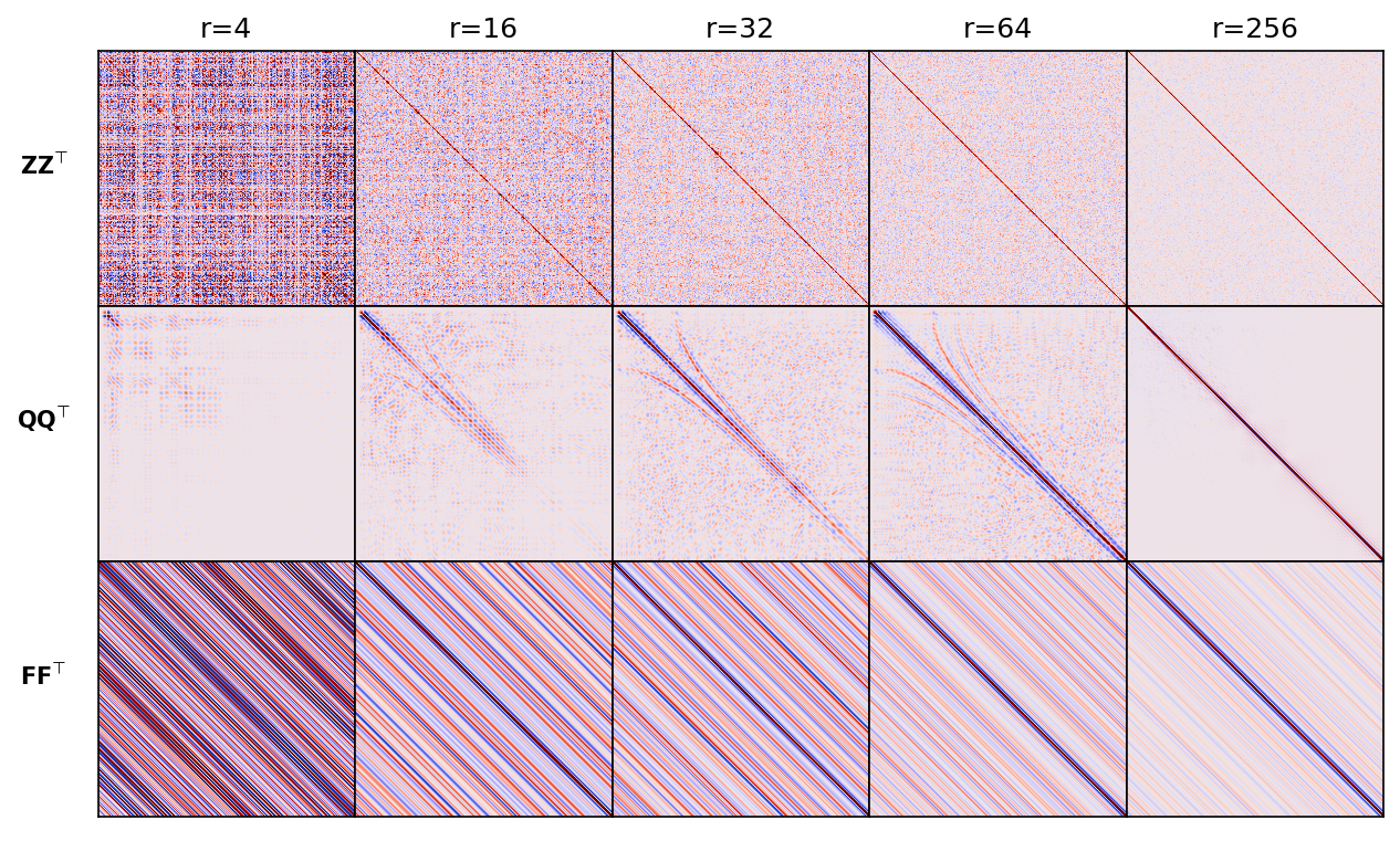
To demonstrate the benefits of the additional orthogonalization step, we include Figure #pvec where comparisons are made between crosstalk produced by probing with Rademacher vectors (Figure #pvec first row); with orthogonalized vectors derived from Rademacher probing according to Equation #QR (Figure #pvec second row); and probing with vectors selected randomly from the Fourier matrix (Figure #pvec third row). The orthogonalized vectors are computed using the same shot record from the 2D overthrust model with ``751`` samples and a ``4``ms sampling rate (``3``sec recording). As expected, the crosstalk---i.e. energy leakage away from the main diagonal, for these different cases varies but decrease with increasing ``r`` for all. However, the frequency content and coherence of the errors do differ. Because the outer product converges the fastest the identity matrix within the seismic frequency band, we argue that the orthogonalized probing vectors perform the best.
#### Figure: {#pvec}
{width=75%}
: Crosstalk for different implementations of randomized probing as a function of increasing probing size ``r=4,\,16,\,32,\,64,\,256``. Compared to probing with Fourier vectors (third column), crosstalk for probing with Rademacher (first column) and orthogonalized Rademacher (second column) is less coherent with energy converging to the main diagonal faster. As expected, this effect is the strongest for the orthogonalized probing vectors within the seismic frequency band.
#### Algorithmic details and validation
Based on the above practical and computational considerations, we propose the implementation as outlined in Algorithm #pic below. This algorithm runs for each source independently (possibly in parallel) and redraws a new probing matrix ``\mathbf{Q}`` for each gradient computation. By propagating the forward wavefield with a single timestep (line 1), ``\operatorname{forward}(\mathbf{u}[t], \mathbf{u}[t-1], \mathbf{m}, \mathbf{q}[t])``, followed by probing with ``r`` vectors (line 2), the second-derivative of the dimensionality reduced forward wavefield is accumulated for each time index (the "for loop" starting at line 2). Notice that we suppressed the loop over the spatial index ``\mathbf{x}``, which is implied. After the forward loop is completed, a similar process is followed when accumulating the dimensionality-reduced adjoint wavefield after back propagation with a single timestep via ``\mathbf{v}[t-1] = \operatorname{backward}(\mathbf{v}[t], \mathbf{v}[t+1], \mathbf{m}, \delta \mathbf{d}[t])``. After the second loop is completed, Algorithm #pic produces an estimate for the trace via ``\frac{1}{r}\operatorname{tr}(\overline{\mathbf{u}}\, \overline{\mathbf{v}}^\top) = \frac{1}{r}\sum_r \overline{\mathbf{u}}[r, :]\odot \overline{\mathbf{v}}[r, :]`` in which use is made of Matlab-style notation.
### Algorithm: {#pic}
| Draw probing matrix ``\mathbf{Q}`` with Equation #QR, set initial condition ``\mathbf{u}[0], \mathbf{u}[1]`` and final conditions ``\mathbf{v}[n_t], \mathbf{v}[n_t-1]``.
| 0. **for ``t=1:n_t-1``** # forward propagation
| 1. ``\mathbf{u}[t+1] = \operatorname{forward}(\mathbf{u}[t], \mathbf{u}[t-1], \mathbf{m}, \mathbf{q}[t])``
| 2. **for ``i=1:r``**
| ``\overline{\mathbf{u}}[i] \pluseq \mathbf{Q}[i, t] \ddot{\mathbf{u}}[t]``
| **end for**
| 3. **end for**
| 4. **for ``t=n_t-1:{-1}:1``** # back propagation
| 5. ``\mathbf{v}[t-1] = \operatorname{backward}(\mathbf{v}[t], \mathbf{v}[t+1], \mathbf{m}, \delta \mathbf{d}[t])``
| 6. **for ``i=1:r``**
| ``\overline{\mathbf{v}}[i] \pluseq \mathbf{v}[t] \mathbf{Q}[i, t]``
| **end for**
| 7. **end for**
| 8. output: ``\frac{1}{r}\operatorname{tr}(\overline{\mathbf{u}}\, \overline{\mathbf{v}}^\top) = \frac{1}{r}\sum_{i=1}^r \overline{\mathbf{u}}[i]\odot \overline{\mathbf{v}}[i]``
: Approximate gradient calculation with random trace estimation
Before reviewing predicted memory savings, let us first make a comparison between single-source gradients computed with the three different probing vectors juxtaposed in Figure #pvec\. To assess the accuracy of results with randomized-trace estimation, we set side by side the approximate gradients as a function of the probing size, ``r=4, 16, 32, 64, 256``, and compare these gradients with the true gradient. We make these comparisons for 2D gradients computed from the overthrust model [@overthrust] with an experimental setting detailed in the Synthetic case studies section below.
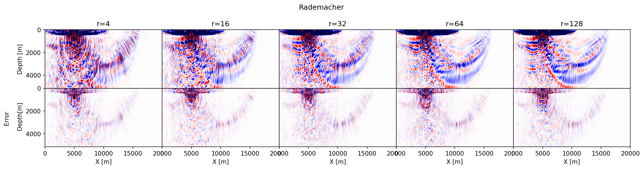
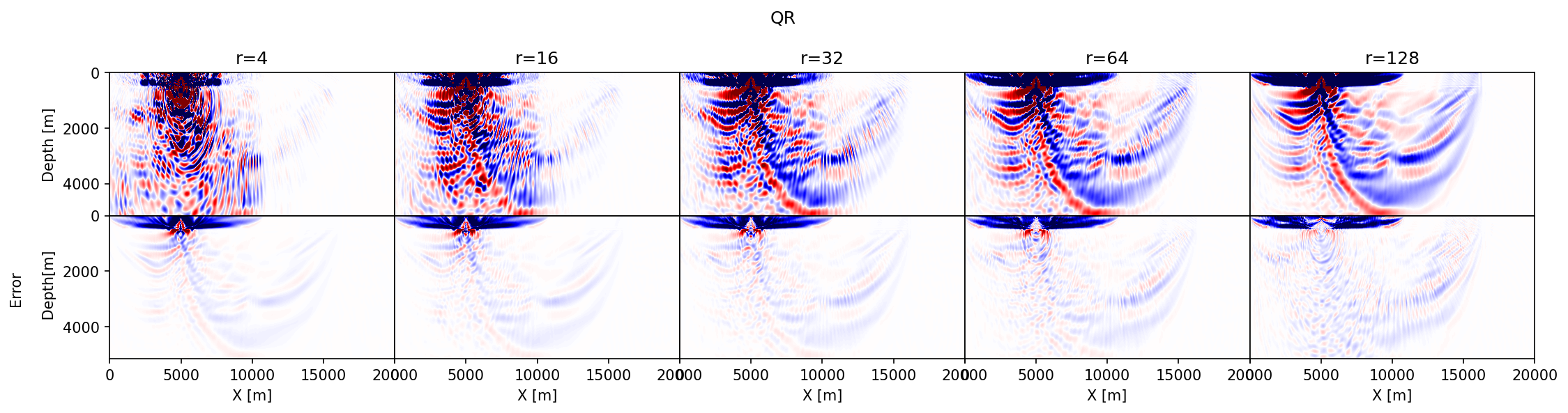
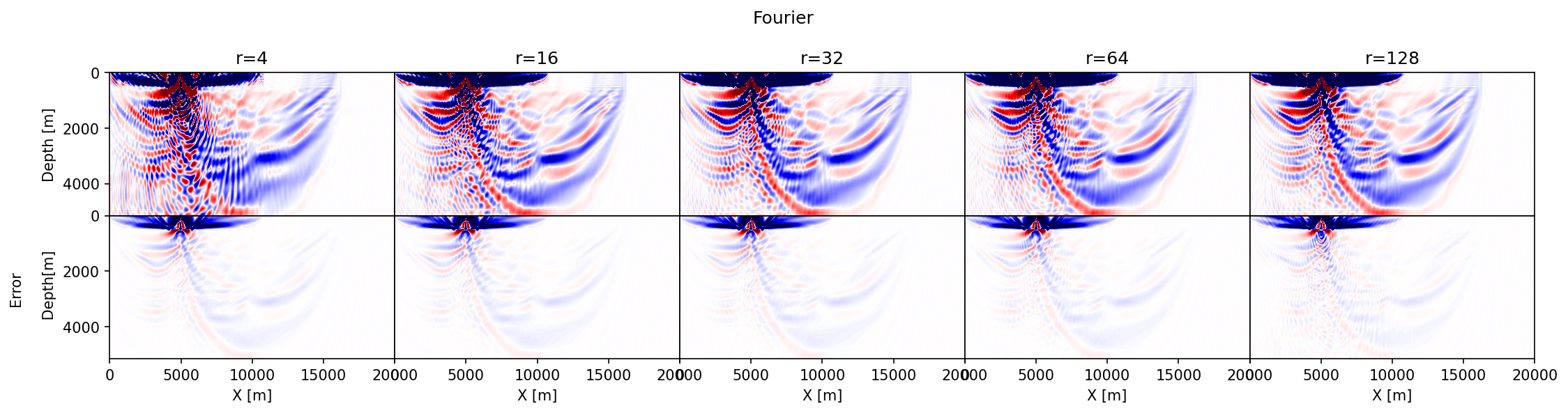
The results of this exercise are summarized in Figure #fig:prob-choice\, which includes difference plots between the true and approximate gradients. The following observations can be made. First, in accordance with the results in Figure #pvec\, the accuracy of the approximate gradient calculations improves for increasing ``r``. Second, probing with Rademacher vectors (Figure #rad) yields gradients that contain noisy relatively high-spatial frequency artifacts that extend across the model and that decay relatively slowly as ``r`` increases. Results obtained with the orthogonalization (Figure #qr) and Fourier (Figure #dft) build up the gradient more slowly as a function of increasing ``r``, capturing the small amplitudes far away from the source only for relatively large ``r``. Because both the orthogonalized and Fourier approaches act within the data's temporal frequency spectrum, they do not contain high-frequency artifacts. Third, as expected results from the orthogonalized probing vectors converge the fastest with the smallest errors. Before conducting more rigorous tests on realistic 2- and 3-D examples, we will first discuss projected memory savings and various extensions involving more elaborate imaging conditions and derived products such as subsurface-offset image volumes.
#### Figure: {#fig:prob-choice}
{#rad width=100%}
{#qr width=100%} \
{#dft width=100%} \
: Comparison between approximate gradients of the 2D overthrust model for a single source and increasing numbers of probing vectors. (a) contains approximate gradients and errors obtained by probing with Rademacher vectors. (b) the same but with orthogonalized Rademacher probing vectors. (c) the same but with probing vectors randomly selected from the Fourier matrix.
### Estimates for the memory footprint
As we mentioned before, excessive memory usage of adjoint-state methods constitute a major impediment to the implementation of wave-based inversion technology on modern accelerators where memory access comes at a premium. For this reason, we proposed approximate calculations with randomized probing where the dimensionality of the forward and adjoint wavefield is reduced by the method described in Algorithm #pic\. Theoretical estimates of the memory imprint can be computed easily from Equation #optr\. We compare these estimates with the memory footprint and computational overhead associated with other low-memory approaches, including optimal checkpointing [@Griewank;@Symes2007;@kukrejacomp]; reconstruction from wavefields on the boundary [@McMechan;@Mittet;@RaknesR45], and the closely related method based on probing with the discrete Fourier transform (DFT) [@Nihei2007;@Sirgue2010;@witte2018cls]. Without loss of generality, we will make these comparisons for the scalar acoustic wave equation in 3D where ``N=N_x \times N_y \times N_z`` is the total number grid points and ``N_x,\, N_y``, and ``N_z`` the number of gridpoints in the ``x-,\, y-``, and ``z-``directions. In that setting, the total memory requirement of conventional FWI is ``N\times n_t`` (single-precision) floating point values, which is prohibitive in practice.
Table #memest lists estimates for memory use and computational overhead to achieve the anticipated memory savings. Values for optimal checkpointing and reconstruction from the boundary are taken from the literature. From these figures, we observe that optimal checkpointing could in principle achieve the largest memory savings at the expense of computational overhead and a relatively complex implementation. While memory savings achieved with the boundary reconstruction method do limit memory usage, this approach scales unfavorably with the number of timesteps, ``n_t``, compared to the methods based on probing with Fourier or the proposed orthogonalized data-adaptive vectors. Because probing with the DFT involves complex numbers, its memory use and computational overhead doubles. Our method, on the other hand, probes with ``\mathbf{Q} \in \mathbb{R}^{n_t \times r}`` and thus requires storage of only ``N\times r`` floating point values during each of the forward and backward passes, which results in a total storage of ``2\times N\times r`` values and a memory reduction by a factor of, ``{n_t}/{2 r}``. This memory reduction corresponds to approximating the gradient with ``\frac{r}{2}`` Fourier modes and puts the DFT approach in a relative disadvantage. Because the errors decay more slowly with ``r`` compared to our randomized-trace method, this drawback is made worse for the Fourier-based method.
### Table: {#memest}
| | FWI
| randomized-trace
| DFT
[@witte2018cls] | Optimal checkpointing
[@Symes2007] | Boundary reconstruction
[@Mittet] |
| :-----: | :---------------: | :-----------------------------------: | :------------------------------------: | :-------------------------------------------: | :----------------------------: |
| Memory | ``N \times n_t `` | ``r \times N`` | ``2r\times N`` | ``\mathcal{O}(\log(n_t)) \times N`` | ``n_t \times N^{\frac{2}{3}}`` |
| Compute | 0 | ``\mathcal{O}(r)\times n_t \times N`` | ``\mathcal{O}(2r)\times n_t \times N`` | ``\mathcal{O}(\log(n_t))\times n_t\times N `` | ``n_t \times N`` |
: Memory estimates and computational overhead of different seismic inversion methods for ``n_t`` time steps and ``N`` grid points. Analytical estimates are extracted from the literature for the methods listed in the table.
Aside from its relative simplicity and favorable (``n_t``-independent) memory scaling, probing methods can, as we will show below, relatively easily be extended to different imaging conditions and vector-valued wave equations. In addition, the proposed method also works for wave propagation in attenuating media, which renders wavefield reconstruction from the boundaries unstable.
## Extensions
In this section, we will show how the proposed randomized probing technique also leads to computationally efficient implementations of more involved imaging conditions including formating of subsurface offset image gathers. Both instances benefit from reductions in computational costs by a factor of ``n_t/r\ll 1``.
### Imaging conditions
So far, we limited ourselves to the scalar isotropic acoustic wave equation with the standard zero-offset imaging condition. While adequate in some applications, seismic imaging and inversion methodologies often call for more sophisticated imaging conditions designed to bring out certain features in migrated images or to make FWI more sensitive to reflections. Because imposing various imaging conditions requires manipulations with the forward and adjoint wavefields, we stand to benefit from replacing these wavefields by their dimensionality reduced counterparts. After incurring the computational overhead of probing, by mapping ``\{\ddot{\mathbf{u}}, \mathbf{v}\} \rightarrow \{\overline{\mathbf{u}}, \overline{\mathbf{v}}\}``, these wavefield manipulations come almost at no additional costs. Below, we showcase a number of illustrative examples that underline this important feature.
#### Spatial differential operations
To improve RTM or FWI, different contributions of the gradient of the adjoint-state method can be (de)emphasized by changing the imaging condition. For instance, tomographic artifacts can be removed from reverse-time migrated images by imposing the inverse scattering imaging condition [@stolk2009inverse;@t2012linearized;@Whitmore;@witteisic]. In a related but different approach, in reflection FWI [@Faqi, @iraborrfwi, @changrfwi], tomographic contributions to the gradient can be emphasized via wavefield separation. As with most imaging conditions, the inverse scattering condition does not entail manipulations along time and involves (differential) operators acting along the spatial coordinates only. Because imaging conditions are often linear, these operations commute with probing, which allows for direct application of imaging conditions on the dimensionality reduced wavefield by using the following identity:
```math {#commute}
\mathbf{Q}^\top \left(\mathbf{D}_x \mathbf{u}[\cdot,\mathbf{x}]\right) = \mathbf{D}_x \left(\mathbf{Q}^\top \mathbf{u}[\cdot,\mathbf{x}]\right)
```
where the symbol ``\mathbf{D}_x`` represents a linear differential operator acting along the spatial coordinates. By virtue of this identity, numerically expensive operations with ``\mathbf{D}_x`` can be factored out, reducing the number of applications of this operator from ``n_t`` to ``r``. Because ``r\ll n_t`` this can lead to significant computational savings, especially in the common situation where imposing imaging conditions may become almost as computationally expensive as solving the wave-equation itself.
#### Subsurface-offset image gathers
Another benefit of approximating gradients via the trace (cf. Equation #optr) is that it makes it possible to compute subsurface-offset image volumes directly on GPUs by working with the dimensionality reduced wavefields---i.e., we have
```math {#ssoffset}
\delta\mathcal{M}[\mathbf{x},\mathbf{h}] \approx \frac{1}{r} \operatorname{tr}\left(\bar{\ddot{\mathbf{u}}}[\cdot, \mathbf{x}+\mathbf{h}]\bar{\mathbf{v}}[\cdot, \mathbf{x}-\mathbf{h}]^\top\right).
```
In this expression, the symbol ``\mathbf{h}`` corresponds to the (horizontal) subsurface offset and ``\delta\mathcal{M}[\mathbf{h}]`` to the subsurface image volume. As with computing the zero-offset imaging condition (Equation #optr), the cost of computing these extended image volumes is reduced by a factor of ``r/n_t``. Finally, note that ``\left.\delta\mathbf{m}[\mathbf{x}]=\delta\mathcal{M}[\mathbf{x},h]\right|_{\mathbf{h}=0}``.
#### Coupled vector-valued wave equation
Adequate representation of the wave physics balanced by computational considerations are prerequisites to the success of seismic inversion on 3D field data. A good example where such a balance is struck is wave modeling with the acoustic tilted transverse isotropic (TTI) wave-equation, where elastic anisotropic behavior of the subsurface is modeled by an acoustic approximation [@thomsen] that is computationally feasible. However, compared to the isotropic scalar acoustic wave equation, the TTI wave-equation requires the solution of two coupled PDEs. Because the gradient with respect to the squared slowness and anisotropic parameters now involves four wavefields, this increases memory pressure. According to [@bubesatti2016;@zhang-tti;@louboutin2018SEGeow], the gradient for the squared slowness in TTI media reads
```math {#ttiim}
\delta\mathbf{m} = \sum_t \ddot{\mathbf{p}}[t]\odot \overleftarrow{\mathbf{p}}[t] + \ddot{\mathbf{r}}[t]\odot \overleftarrow{\mathbf{r}}[t] = \operatorname{tr}(\ddot{\mathbf{p}} \overleftarrow{\mathbf{p}}^\top) + \operatorname{tr}(\ddot{\mathbf{r}} \overleftarrow{\mathbf{r}}^\top)
```
where ``\mathbf{p}`` and ``\mathbf{r}`` are solutions of two coupled PDEs and ``\overleftarrow{\mathbf{p}}`` and ``\overleftarrow{\mathbf{r}}`` are solutions of the adjoint of these coupled PDEs. When implemented naively, the memory footprint would effectively double when the above gradients are approximated with separate randomized-trace estimations for ``\ddot{\mathbf{p}}[t] \odot \overleftarrow{\mathbf{p}}[t]`` and ``\ddot{\mathbf{r}}[t] \odot\overleftarrow{\mathbf{r}}[t]``\. However, these extra costs can be avoided if we make use of the following identity:
```math {#trequi}
\operatorname{tr}(\ddot{\mathbf{p}} \overleftarrow{\mathbf{p}}^\top) + \operatorname{tr}(\ddot{\mathbf{r}} \overleftarrow{\mathbf{r}}^\top) = \operatorname{tr}(\Vect{\ddot{\mathbf{p}}}{\ddot{\mathbf{r}}} \Vect{\overleftarrow{\mathbf{p}}}{\overleftarrow{\mathbf{r}}}^\top),
```
which holds for the trace of vector-valued wavefields. When cast in this form, the above gradient can be approximated by
```math {#eq:vectrace}
\delta\mathbf{m} = \operatorname{tr}(\Vect{\ddot{\mathbf{p}}}{\ddot{\mathbf{r}}} \Vect{\overleftarrow{\mathbf{p}}}{\overleftarrow{\mathbf{r}}}^\top) &\approx \frac{1}{r} \operatorname{tr}(\Vect{\mathbf{Q}}{\mathbf{Q}}^\top \Vect{\ddot{\mathbf{p}}}{\ddot{\mathbf{r}}} \Vect{\overleftarrow{\mathbf{p}}}{\overleftarrow{\mathbf{r}}}^\top \Vect{\mathbf{Q}}{\mathbf{Q}}) \\
&\approx \frac{1}{r} \operatorname{tr}\left((\mathbf{Q}^\top (\ddot{\mathbf{p}}+\ddot{\mathbf{r}})) ((\overleftarrow{\mathbf{p}}+\overleftarrow{\mathbf{r}})^\top \mathbf{Q})\right)
```
if the same probing vectors are used for each component of the vector-valued wavefield. Using this expression reduces the memory cost to that of a single probed wavefield and consequently its memory use remains the same as that of gradients of isotropic acoustic media, which we consider as a major advantage or our method. In practice, we observe that the accuracy of this approximation does not decrease when the same probing matrix ``\mathbf{Q}`` is used. With significant computational and memory savings established, we will now validate its performance on realistic numerical experiments of varying complexity and problem size.
## Numerical case studies
While the presented methodology has the potential to unlock usage of memory-scarce accelerators, its performance needs to be validated on realistic wave-equation based inversion examples. For this purpose, we consider three synthetic examples that vary in complexity of the wave physics. First, we revisit the 2D overthrust model and compare conventional FWI results with inversions obtained with randomized-trace estimation for increasing numbers of probing vectors. In the second example, we demonstrate that our probing method is capable of producing high-quality subsurface-offset image volumes at significantly reduced computational cost. We conclude by showcasing a 3D FWI example. We limit our considerations to synthetic data because it allows us to make informed comparisons between exact and approximate gradient calculations.
## 2D Full-waveform inversion
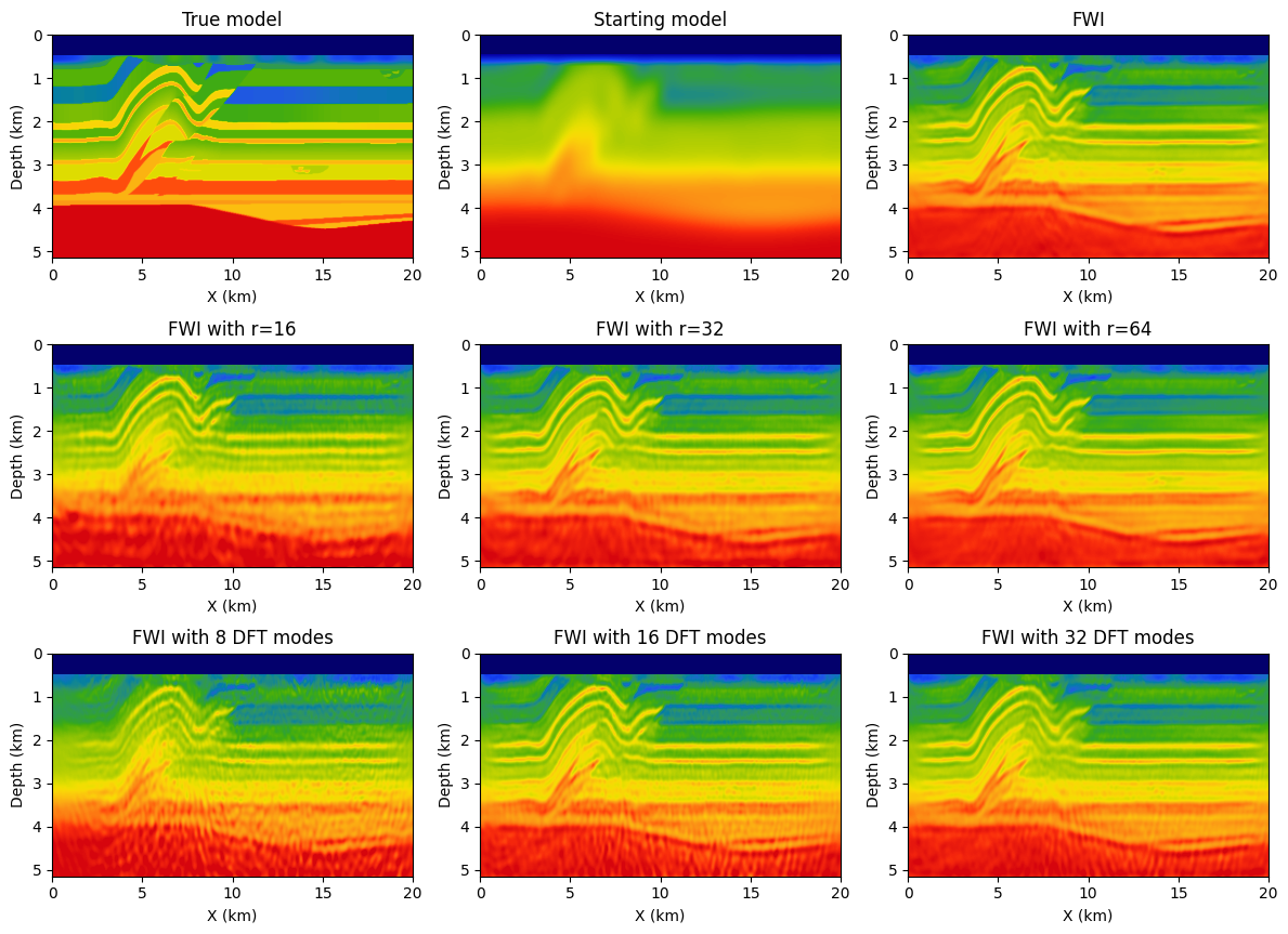
As part of validating our random-trace estimation technique, we consider a synthetic 2D acoustic FWI example with a geometry representing a sparse OBN acquisition while applying source-receiver reciprocity (coarse sources, dense receivers). The data is simulated for a ``20``km by ``5``km section taken from the overthrust model [@overthrust] and plotted in Figure #fig:2d-fwi-comp-sm top left. For the FWI experiment, we work with ``97`` shot records sampled ``200``m apart, mimicking sparse OBNs sampled at one source position per wavelength. Each shot record contains between ``127`` and ``241`` receivers ``50``m apart, yielding a maximum offset of ``6``km. The data is modeled with a ``8``Hz Ricker wavelet and ``3``sec recording.
For reference, we first conduct conventional FWI given the smooth starting model depicted in Figure #fig:2d-fwi-comp-sm top middle. We compare this conventional FWI result plotted in Figure #fig:2d-fwi-comp-sm top tight with results yielded by approximate gradient calculations where the memory footprint is kept the same experiment by experiment---i.e., ``r=16,\, 32,\, r=64`` for randomized-trace estimation with orthogonalized probing vectors, and ``8,\, 16,\, 32`` for probing with randomly selected Fourier modes. Results of these experiments are included in the second and third row of Figure #fig:2d-fwi-comp-sm\. In all cases, FWI results are computed with ``20`` iterations of the Spectral Projected Gradient method (SPG, @schmidt09a), which imposes box and total-variation (TV) constraints on the inverted velocity model. Computational costs are limited by working with subsets of ``8`` randomly selected (without replacement) shots [@Aravkin11TRridr]. From the approximations plotted in Figure #fig:2d-fwi-comp-sm\, we can make the following observations. First, compared to results obtained with ``16`` Fourier modes our result for the same number of probing vectors contains fewer coherent steeply dipping artifacts especially at deeper areas of the inverted velocity model. Second, when memory use is kept constant, e.g. by choosing ``r=32`` orthogonalized probing vector and ``16`` complex-valued DFT modes, our method produces results that are more accurate and less noisy. This observation is consistent with results presented in Figure #pvec\.
#### Figure: {#fig:2d-fwi-comp-sm}
{width=100%}
: Comparison of FWI on the 2D overthrust model between our proposed probed method with ``16``, ``32``, and ``64`` orthogonalized probing vectors and results obtained with on-the-fly DFTs with an equivalent memory imprint, which corresponds to ``8``, ``16``, and ``32`` Fourier modes.
## 2D extended TTI imaging
To illustrate our ability to handle more realistic physics, we show that it is possible to create high-fidelity subsurface-offset image gathers with the proposed randomized-trace estimation technique. For this purpose, shot data provided with 2007 BP TTI model is migrated using our randomized approximation. The resulting image---i.e., the zero offset/angle section, is shown in Figure #fig:2d-bp-sso and shows accurate location and continuity of reflectors compared to the existing literature [@lrttirtm;@louboutin2018SEGeow]. We also computed subsurface image gathers using the approximation given in Equation #eq:vectrace\. We show the computed subsurface-offset image gather in Figures #fig:2d-bp-sso-og and corresponding subsurface-angle gathers in Figure #fig:2d-bp-sso-ag\. Even though only a limited number of probing vectors (``r=64\ll n_t``) were used, the resulting image gathers are properly focused and nearly noise-free thanks to the relatively high fold. Each image volume, of size ``n_x \times n_y \times n_{\text{offsets}}``, consists of ``81`` offsets between ``-500`` and ``500m`` sampled at ``12.5m``. Remark that formation of these image volumes requires more memory, namely ``81`` model-size arrays, than carrying out the probing itself, which involves only ``64`` model-size probed wavefields for ``\overline{\mathbf{u}}, \overline{\mathbf{v}}``). This highlights how memory frugal our proposed randomized-trace estimation method really is.
#### Figure: {#fig:2d-bp-sso}
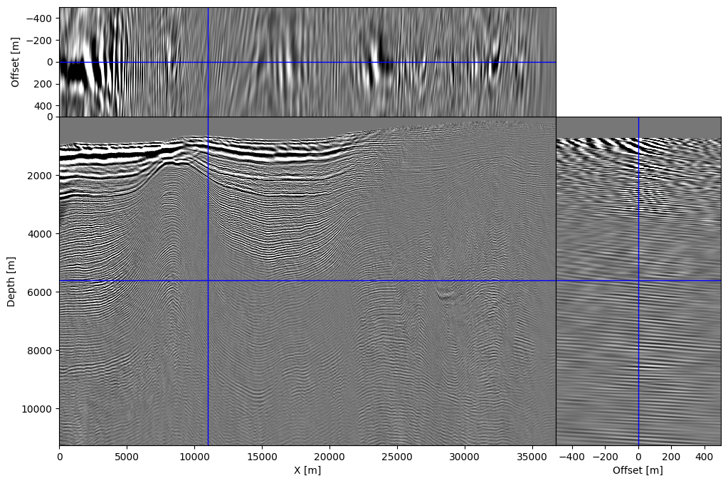{width=45% #fig:2d-bp-sso-og}
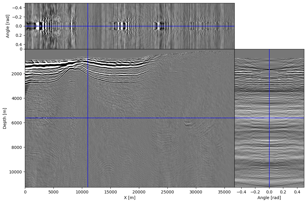{width=45% #fig:2d-bp-sso-ag}
: Subsurface offset (a) and angle b) gathers with ``-500m`` to ``500m`` horizontal subsurface offset and ``-.5rad`` to ``.5rad`` subsurface angles.
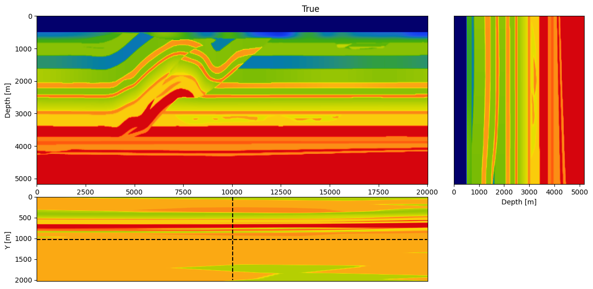
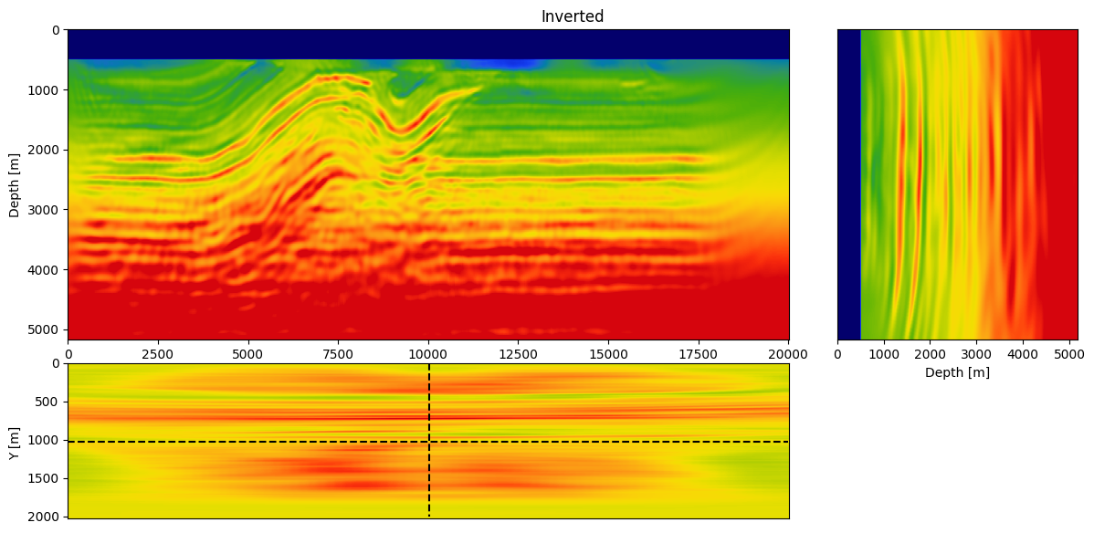
## 3D full-waveform inversion
Finally, to demonstrate scalability we run 3D FWI on the overthrust model. The computational resources needed for this inversion exceeds available memory on Azure's Standard_NC6 instances whose NVIDIA K80 GPUs are limited to ``8``Gb each, rendering FWI implementations without checkpointing/offloading/streaming impractical. Because our method only requires a fraction of memory, we are actually able to run 3D FWI with randomized-trace estimation (for ``r=64\ll n_t``) on 50 instances.
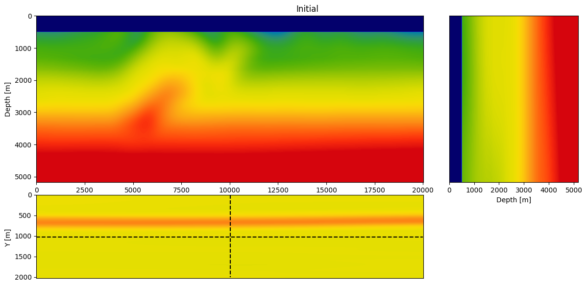
Specifically, we consider a narrow azimuth towed streamer acquisition on a `20`km X `2km` X `5km` (inline X crossline X depth) subsection of the Overthrust model. The acquisition consists of ``1902`` sources (50m inline spacing and 200m crossline spacing) with six ``8km`` long cables ``100m`` apart with a receiver spacing of ``12.5m`` per. We simulate the shot data with a ``12.5Hz`` Ricker wavelet. To avoid unrealistic low frequencies, frequencies below ``3Hz`` are removed with a high-pass filter. Given these simulations, ``20`` iterations of FWI are performed using ``r=32`` orthogonalized probing vectors and ``400`` sources per iteration. As before, FWI is carried out with projected quasi-Newton (PQN, @schmidt09a) imposing both box and TV constraints [@peters2018pmf;@petersmink]. The box constraints guarantee physical velocities while the TV constraint removes noisy artifacts due to the randomized-trace estimation. The inverted velocity model is included in Figure #fig:3d-fwi\.
#### Figure: {#fig:3d-fwi}
{#init width=100%} \
{#init width=100%} \
{#probed width=100%}
: 3D FWI of the 3D overthrust model on Azure using 50 K80 (NVIDIA Kepler, 8Gb memory) nodes. The inversion was performed with 32 probing vectors (``r=32``), which approximate each gradient natively on the GPUs without relying on any form of checkpointing.
From this experiment, we see that we recover an accurate velocity model that contains most of the main features of the true model and recovered most of the fine layers at depth. This result shows that the proposed method scales to realistic 3D model without the need for additional probing vectors to compensate for the additional dimension (compared to the 2D FWI result).
### Code availability
Our implementation and examples are available as open-source software at [TimeProbeSeismic.jl], which extends our Julia inversion framework [JUDI.jl][@witteJUDI2019;@judi]. Our code is also designed to generalize to 3D and more complicated physics as supported by [Devito][@devito-api;@devito-compiler;@devito].
## Discussion and conclusions
By approximating the gradient of wave-based inversion with randomized trace estimation, we were able to drastically reduce the memory footprint of time-domain full-waveform inversion and reverse-time migration with the adjoint-state method. Through careful design of data-adaptive probing vectors, memory reductions between ``20\times`` and ``100\times`` were achieved without tangible loss in accuracy. These attained memory reductions, in turn, facilitate accelerator-native software implementations for the time-domain adjoint-state method, which benefit maximally from graphics processing units with limited computational overhead. To achieve these results, we controlled the approximation errors due to randomized-trace estimation by increasing the number of probing vectors, the fold, and by imposing additional constraints, e.g. the total-variation norm, during inversion. Because of its relatively simplicity, the proposed method can be extended readily to more complicated wave physics, including vector-valued wavefields in transversely isotropic media. By virtue of the memory footprint reduction, the proposed method is also capable of efficient calculation of extended (subsurface-offset) image volumes with computational gains that are proportional to the reductions in memory usage. In future work, we plan to expand this work to include extended Born least-squares migration and extended full-waveform inversion.
## Acknowledgement
This research was carried out with the support of Georgia Research Alliance and partners of the ML4Seismic Center. We thank John Washbourne for the constructive discussions.
[TimeProbeSeismic.jl]:https://github.com/slimgroup/TimeProbeSeismic.jl
[JUDI.jl]:https://github.com/slimgroup/JUDI.jl
[Devito]:https://www.devitoproject.org
```math_def
\newcommand{\pluseq}{\mathrel{+}=}
\newcommand{\Vect}[2]{\ensuremath{\begin{bmatrix} #1 \\ #2 \end{bmatrix}}}
```