Target-oriented imaging using extended image volumes—a low-rank factorization approach

Rajiv Kumar^1,2, Marie Graff-Kray¹, Ivan Vasconcelos³ and Felix J. Herrmann^1,2
1 Seismic Laboratory for Imaging and Modeling (SLIM), the University of British Columbia
² Georgia Institute of Technology, USA
³ Utrecht University, the Netherlands 

Introduction

Seismic data are the primary source of information used to image structures, evaluate rock properties, and monitor their changes in the Earth’s subsurface. To achieve these goals, seismic reflection imaging relies on kinematically correct background-velocity models. However, imaging from acquired data struggles to reveal the true location of the subsurface reflectors at the deeper sections, particularly in geological environments presenting complex overburden structures such as high-velocity salt bodies or low-velocity gas chimneys. This is due to the fact that the existing ray-based imaging methods cannot adequately describe the wave propagation in complex geological scenarios and sophisticated wave-equation based methods are very sensitive to the accuracy of the near-surface or overburden velocity model.

The seismic community proposed various methods to overcome these difficulties. These methods can be divided into two-main categories. The first method is called virtual source technology (Bakulin et al., 2004, 2008), where borehole seismic data is acquired with receivers being deployed beneath the complex part of the overburden and sources are placed at the surface. Virtual source data at the receivers locations are created using time reversal techniques applied to the surface-to-downhole data, where time-gated data are passed through the time reversal process and convolved with the surface-to-downhole data. The resulting virtual source data are then imaged with conventional methods using the velocity information below the receivers. Although this method is beneficial for removing artifacts caused by the complex overburden, it requires receivers to be placed in the borehole, which is not practical in exploration surveys.

The second method is called interferometric redatuming, which has been studied extensively in the literature (Snieder, 2004; Wapenaar and Fokkema, 2006; Schuster and Zhou, 2006; Snieder et al., 2006; Mehta et al., 2007; Schuster, 2009; Curtis and Halliday, 2010; Broggini et al., 2012; Wapenaar et al., 2012; van der Neut and Herrmann, 2013). In interferometric redatuming, seismic data are acquired by placing both sources and receivers at the surface during the acquisition. Then a virtual seismic response at the subsurface datum is created by performing a multidimensional deconvolution of the upgoing waves with respect to the downgoing waves, where the downgoing and upgoing wave constituents are created from the transmitted waves by inverting the model-based wavefield composition matrix (Schuster and Zhou, 2006 Wapenaar et al. (2008)). One drawback of this method is that one has to invert this composition matrix, which can be challenging because it exhibits singularities at critical angles. We can overcome this by regularizing the least-square solutions to generate the down- and upgoing wavefields as shown in van der Neut and Herrmann (2013), where the authors proposed to solve a sparsity-promotion based least-squares formulation. Alternatively, Wapenaar and van der Neut (2010); Vasconcelos and Rickett (2013) proposed multidimensional deconvolution based imaging conditions using extended image volumes, where two-way wave-equation based extrapolation is used to generate the full nonlinear reflection response at a given target-datum in the subsurface, as a function of time or frequency.

Although, multidimensional deconvolution based imaging conditions using extended image volumes have shown potential benefits in target-oriented imaging (van der Neut and Herrmann, 2013; Vasconcelos and Rickett, 2013; Ravasi et al., 2016), evaluating these reflection responses is prohibitively expensive in realistic (3D) settings. This is due to the fact that it involves solving two-way wave-equation extrapolation with a conventional shot-profile approach at any particular datum in the subsurface. For the conventional shot-profile approach, the required number of partial differential (wave) equation (PDE’s) evaluations is equal to twice the number of sources. Since, we need to solve so many PDE’s, the use of conventional two-way approaches to perform target-oriented imaging is very expensive especially for industrial scale problems in 2D and 3D. To overcome these computational costs, we first analyze the algebraic structure of full subsurface extended image volumes organized as a matrix. Here, each column of this matrix represents a source experiment that captures the reflection response in both horizontal as well as vertical directions since it is derived from the two-way wave-equation (Berkhout, 1992; van Leeuwen et al., 2015). We find that monochromatic full subsurface extended image volumes exhibit a low-rank structure for low-to-mid range frequencies. If we can somehow gain access to this low-rank structure, we will be able to reduce the number of required PDE solves to a number that is proportional to the rank and not the number of sources. To accomplish this, we propose a framework using randomized singular value decomposition (Halko et al., 2011) that gives us the needed low-rank factorization of full subsurface extended image volumes. Following van Leeuwen et al. (2015), we build this low-rank factorization representation using matrix-free operations with probing vectors that cost only two PDE solves per vector. The randomized singular value decomposition with probing techniques also helps us to mitigate the costs of two-way wave-equation solves and multi-dimensional deconvolutions. Apart from the computational cost, the low-rank factorization also drastically reduces the memory storage, which one incurs in conventional shot-profile approaches.

The paper is organized as follows: we begin by introducing the multi-dimensional deconvolution-based extended imaging conditions in a two-way wave-equation setting. Next, we show a computationally affordable and memory-efficient way of computing the reflection response at a subsurface datum using probing techniques. We illustrate these features on a small section of the Marmousi model for which we can form the matrices for comparison and we show that our low-rank approach is in principal scalable with the model size. On a larger more complex model, we carry out our redatuming and show that we are able to handle the low-velocity zone in the overburden. Although, probing techniques overcome an important computational bottleneck, we only have very limited access to the full subsurface reflection response because we are restricted to the physical locations of the probing vectors. To get access to the full subsurface image volume for all subsurface points, we propose to take the randomized singular value decomposition with probing a step further by representing the image volumes themselves in a low-rank factored form. Finally, we demonstrate the computational advantages of low-rank factored form to perform the target-oriented imaging beneath the salt using a section of Sigsbee2A model (The SMAART JV (2001)).

Extended image volumes via deconvolution

Before we describe the proposed methodology of extracting the target-oriented reflection response from full subsurface extended image volumes, we first review the governing equations. Given the time-harmonic source and receiver wavefields, denoted by \(u({\bf{x}},{\bf{x}}_s,\omega)\) and \(v({\bf{x}}',{\bf{x}}_s,\omega)\), the reflection response \(r\) (Berkhout, 1992; Vasconcelos et al., 2010; Thomson, 2012) of the medium below the datum \(\partial D_d\) satisfies the following relationship \[ \begin{equation} v({\bf{x}}',{\bf{x}}_s,\omega)= \int_{{\bf{x}}\in\partial D_d} r({\bf{x}}',{\bf{x}},\omega)u({\bf{x}},{\bf{x}}_s,\omega) {\mathrm{d}}^2{\bf{x}}, \label{refm} \end{equation} \] where \(\mathbf{x},{\mathbf{x}}'\in \mathcal{D} \subset \mathbb{R}^n\) (\(n=2\) or \(3\)) represent any subsurface position, \(\omega \in \Omega \subset \mathbb{R}\) is the temporal frequency and \({\mathbf{x}}_s \in {\mathcal{D}}_s \subset \mathbb{R}^{n-1}\) the location of sources deployed at the surface. For more details on how to derive the subsurface reflection response in the acoustic case, we refer to Wapenaar and van der Neut (2010). The source and receiver wavefields are obtained by solving the following two-way wave-equations \[ \begin{equation} \begin{aligned} H(m)u(\mathbf{x},{\mathbf{x}}_s,\omega) &=& q(\mathbf{x},{\mathbf{x}}_s,\omega),\\ H(m)^*v({\mathbf{x}}',{\mathbf{x}}_s,\omega) &=& \int_{{\mathcal{D}_r}}{\mathrm{d}{\mathbf{x}}_r}d({\mathbf{x}}_r,{\mathbf{x}}_s,\omega)\delta({\mathbf{x}}'-{\mathbf{x}}_r), \end{aligned} \label{wave} \end{equation} \] where \(H(m) = \omega^2 m(\mathbf{x})^2 + \nabla^2\) is the Helmholtz operator with Sommerfeld boundary conditions, \(m\) the squared slowness, the symbol \(^*\) represents the conjugate-transpose, \(q\) denotes the source function and \(d\) the reflection-data at receiver positions \({\mathbf{x}}_r \in{\mathcal{D}}_r\subset {\mathbb{R}}^{n-1}\).

To do numerical computations, we discretize our domain of interest \(\mathcal{D}\) with a rectangular grid with a total of \(N_x\) grid points. We will denote \(N_s\) the number of sources, \(N_r\) the number of receivers and \(N_f\) the number of frequencies. The discretized source and receiver wavefields \({{\mathbf{U}}}\) and \({{\mathbf{V}}}\) become 3D tensors of size \(N_x \times N_s \times N_f\). For the \(i^{th}\) frequency, \({{\mathbf{U}}}_i\) and \({{\mathbf{V}}}_i\) represent complex valued source and receiver wavefields organized as \(N_x \times N_s\) matrices, where each column of these matrices contains a monochromatic source experiment. The reflection response can also be expressed as a 3D tensor \({{\mathbf{R}}}\) of size \(N_x \times N_x \times N_f\), where a slice \({{\mathbf{R}}}_i\) at the \(i^{th}\) frequency is a \(N_x \times N_x\) matrix, which satisfies \[ \begin{equation} \mathbf{V}_i = \mathbf{R}_i\mathbf{U}_i \label{ref} \end{equation} \] The discrete form of equation \(\eqref{wave}\) is then obtained by solving \[ \begin{equation} \begin{aligned} \mathbf{U}_i &= \mathbf{H}_i(\mathbf{m})^{-1}\mathbf{P}_s^T\mathbf{Q}_i,\\ \mathbf{V}_i &= (\mathbf{P}_r\mathbf{H}_i(\mathbf{m})^{-1})^{*}\mathbf{D}_i, \end{aligned} \label{wavedis} \end{equation} \] where \({\mathbf{H}}_i\) is a discretization of the two-way Helmholtz operator \((\omega_i^2 \mathbf{m} + \nabla^2)\) for temporal frequency \(\omega_i\) and for a gridded squared slowness \(\mathbf{m}\). We use the notations \(^\ast\) for the conjugate-transpose, \(^{-\ast}\) for its inverse, and \(^T\) for the transpose. Each column of the \(N_s \times N_s\) matrix \({\mathbf{Q}}_i\) represents the discretized source function, and the \(N_r \times N_s\) matrix \({\mathbf{D}}_i\) contains the monochromatic observed wavefields after removing the direct wave and source and receiver side ghosts. Matrices \({\mathbf{P}}_s\) and \({\mathbf{P}}_r\) sample the wavefields at the source and receiver positions. Their transpose injects the sources and receivers wavefields into the grid at the source and receiver locations. For the sake of simplicity, we drop the frequency index \(i\) for the remainder of paper.

To perform the target-oriented imaging, we need access to the reflection response \({{\mathbf{R}}}\) at the subsurface datum \(\partial{D}\) of interest for given source and receiver wavefields. Because \({{\mathbf{U}}}\) is not a full-rank (the maximum rank of \({{\mathbf{U}}}\) is \(N_s\)), we can not straightforwardly compute its inverse to calculate \({{\mathbf{R}}}\). For this reason, we compute the subsurface reflection response \({{\mathbf{R}}}\) in the least-squares sense as follows: \[ \begin{equation} \underset{{\mathbf{R}}}{\text{minimize}} \quad \frac{1}{2} \| {{\mathbf{V}}} - {\mathbf{RU}}\|_F^2, \label{ref1} \end{equation} \] where \(\|\mathbf{A}\|_F^2 = \sum_{i,j}|a_{i,j}|^2\) denotes the Frobenius norm squared. One way to solve equation \(\eqref{ref1}\) is by cross-correlating both sides of equation \(\eqref{ref}\) with \({\mathbf{U}}\), which results in the following normal equation \[ \begin{equation} \mathbf{\underbrace{\mathbf{{VU}}{^*}}_{\mathbf{E}}} = {\mathbf{R}}\mathbf{\underbrace{({\mathbf{U}}{\mathbf{U}}{^\ast})}_{\mathbf{\Gamma}}}. \label{ref3} \end{equation} \] Here, \[ \begin{equation*} \mathbf{E} = \mathbf{{VU}{^\ast}} = {\mathbf{H}}^{-\ast}{\mathbf{P}}_r^{T}\mathbf{DQ}^{\ast}{\mathbf{P}}_s{\mathbf{H}}^{-*} \end{equation*} \] represents the monochromatic extended image for all subsurface offsets and for all subsurface points computed as the cross-correlation between the source and receiver wavefields, whereas \[ \begin{equation*} \mathbf{\Gamma} = \mathbf{UU}{^\ast} = {\mathbf{H}}^{-1}{\mathbf{P}}_s^{T}\mathbf{QQ}^{\ast}{\mathbf{P}}_s{\mathbf{H}}^{-\ast} \end{equation*} \] corresponds to the monochromatic wavefield point-spread function (PSF), which can be seen as the radiation pattern of the virtual sources (van der Neut et al., 2010). Both \(\mathbf{E}\) and \(\mathbf{\Gamma}\) are matrices of size \(N_x \times N_x\). Given the above relationship, \(\mathbf{E}\) can be interpreted as a defocusing (lower resolution) of the reflection response \({\mathbf{R}}\) by the PSF function \(\mathbf{\Gamma}\) for all subsurface offsets and for all subsurface points that lie on the subsurface datum \(\partial D_d\).

To retrieve \({\mathbf{R}}\) from equation \(\eqref{ref3}\), we need to compute the inverse of \(\mathbf{\Gamma}\) and apply it as a filter to the cross-correlated source and receiver wavefields \(\mathbf{E}\). This filtering process to recover the focused \({\mathbf{R}}\) is known as multidimensional deconvolution (MDD) (Wapenaar et al., 2008). Opposed to cross-correlation (Wapenaar and Fokkema, 2006), the retrieval of \({\mathbf{R}}\) with multidimensional deconvolution (Herrmann and Wang, 2008; Wapenaar and van der Neut, 2010), compensates for illumination, finite aperture, and intrinsic losses, etc. In classical settings, the process to generate the reflection response at the subsurface datum \(\partial D_d\) corresponds to the following steps, (i) solve the wave-equation twice for each surface source to calculate the \({\mathbf{U}}\) and \({\mathbf{V}}\) matrices, respectively, (ii) perform the cross-correlations as per equation \(\eqref{ref3}\) to generate \(\mathbf{E}\) and \(\mathbf{\Gamma}\), (iii) perform the MDD in the least-squares sense to retrieve \({\mathbf{R}}\). As a consequence, we have to solve the wave-equation for all sources and receivers within the seismic survey to compute the reflection response at a particular datum in the subsurface. This operation can easily become computationally and storage wise too expensive even for relatively small 2D cases.

To overcome the computational cost of calculating a least-squares estimate for \({\mathbf{R}}\) at a particular datum in the subsurface, we follow the probing technique proposed by van Leeuwen et al. (2015). This technique is designed to perform matrix-free operations to extract information from matrices that can not be formed explicitly because they are too big and dense. In this way, we remove most of the computational and storage requirements to work with the full-subsurface extended image volumes. Following van Leeuwen et al. (2015), in order to probe we multiply equation \(\eqref{ref3}\) from the right by a tall \(N_x \times K\, (K\ll N_x)\) probing matrix \(\mathbf{W} = [{\bf{w}}_1, \ldots, {\bf{w}}_{K}]\) yielding \[ \begin{equation} \begin{split} \mathbf{\widetilde{E}} = \mathbf{EW} = {\mathbf{H}}^{-*}{\mathbf{P}}_r^{T}\mathbf{DQ}^{*}{\mathbf{P}}_s{\mathbf{H}}^{-*}\mathbf{W}, \\ \\ \widetilde{\mathbf{\Gamma}} = \mathbf{\Gamma W} = {\mathbf{H}}^{-1}{\mathbf{P}}_s^{T}\mathbf{QQ}^{*}{\mathbf{P}}_s{\mathbf{H}}^{-*}\mathbf{W}. \\ \end{split} \label{prob} \end{equation} \] In this expression, \(K\) is the number of probing vectors. We denote probed quantities by the symbol \(\widetilde{\cdot}\). For redatuming, we chose the columns \(\mathbf{W}\), \({\bf{w}}_j\) for \(j = 1...K\), to be given by \({\bf{w}}_j = [0, \ldots, 0, 1, 0,\ldots, 0]\)—i.e., a vector containing a single point scatterer at the \(j^{th}\) grid location. By virtue of this choice, the \({\mathbf{w}}_j\) plays the role of a point source located at the datum of interest \(\partial D_d\). As a result of this type of probing, each column of \(\mathbf{\widetilde{E}}\) represents a common-image point (CIP) gather and each column of \(\mathbf{\widetilde{\Gamma}}\) represents the source-side blurring kernel at the subsurface locations corresponding to the \({\bf{w}}_j\)’s. In Algorithm 1, we describe how to compute \(\mathbf{\widetilde{E}}\) and \(\mathbf{\widetilde{\Gamma}}\) in a computationally efficient manner.

1. Inputs – source matrix \(\mathbf{Q}\) , data matrix \(\mathbf{D}\) , and probing matrix \(\mathbf{W}\)
2. Outputs – probed extended image volume \(\widetilde{\mathbf{E}}\), and probed point-spread function \(\widetilde{\mathbf{\Gamma}}\)
3. compute \({\mathbf{\widetilde{U}}} = {\mathbf{H}}^{-*}\mathbf{W}\) and sample this wavefield at the source locations \(\mathbf{\widetilde{D}} = {\mathbf{P}}_s\widetilde{\mathbf{U}}\),
4. correlate the results with source function \(\mathbf{\widetilde{Q}} = {\mathbf{Q}}^*\mathbf{\widetilde{D}}\),
5. use the result as data weights \(\widetilde{{\mathbf{L}}_1} = {\mathbf{D}{\mathbf{\widetilde{Q}}}}\) and \(\widetilde{{\mathbf{L}}_2} = {{\mathbf{Q}}^{*}{\mathbf{\widetilde{Q}}}}\),
6. inject the wavefield \(\widetilde{{\mathbf{L}}_1}\) at the receiver locations and compute the extended image as \({\mathbf{\widetilde{E}} = {\mathbf{H}}^{-*}{\mathbf{P}}_r^T\widetilde{{\mathbf{L}}_1}}\),
7. inject the wavefield \(\widetilde{{\mathbf{L}}_2}\) at the source locations and compute the PSF as \(\widetilde{\mathbf{\Gamma}} = {\mathbf{H}}^{-1}{\mathbf{P}}_s^T\widetilde{{\mathbf{L}}_2}\).

Now that we have access to probed versions of the relevant quantities (\(\mathbf{\widetilde{E}}\) and \(\mathbf{\widetilde{\Gamma}}\)), we are now in a position to determine the reflection response from the relation: \(\mathbf{\widetilde{E}} = \mathbf{\widetilde{R}}\mathbf{\widetilde{\Gamma}}\). Note that compared to the earlier expressions, the matrix \(\widetilde{\mathbf{R}}\) only contains the reflection response restricted to the datum of interest \(\partial D_d\) probed by \(\bf{W}\). As before, we need to compute the inverse of \(\mathbf{\widetilde{\Gamma}}\) to compute \({\mathbf{\widetilde{R}}}\) . Since \(\mathbf{\widetilde{\Gamma}}\) is rank deficient with a maximum rank of \(K\), we compute the reflection response via \[ \begin{equation} \mathbf{\widetilde{R}} = \mathbf{\widetilde{E} \widetilde{\Gamma}}^{\ddagger}; \label{fin} \end{equation} \] where \(^\ddagger\) represents the damped Moore-Penrose pseudo-inverse. After applying this pseudo inverse, each column of \(\mathbf{\widetilde{R}}\) now contains a common-image point (CIP) gather after source-side deblurring at the subsurface locations represented by the \({\bf{w}}_j\)’s located on the datum of interest \(\partial D_d\). To summarize, target-oriented imaging involves the following steps: (i) compute \(\mathbf{\widetilde{R}}\) at a given datum \(\partial D_d\) using equation \(\eqref{fin}\) for each frequency; (ii) take the inverse Fourier-transform along the time-axis to get the time-domain reflection response; and (iii) perform time-domain reverse time-migration to generate the image in the area of interest below the datum \(\partial D_d\). Before we demonstrate the validity of this approach, let us first make a detailed comparison of the computational costs of our approach versus those that use more traditional techniques.

Computational Aspects

The key contribution of this work lies in illustrating the advantages probing techniques have compared to the cost involved on methods that only rely on MDD’s. For this purpose, we compare the computational cost and memory usage of calculating the reflection response at a single scattering point at the datum \(\partial D_d\) somewhere in the subsurface. As we can see from Algorithm 1, solving the wave-equation constitutes the main computational bottleneck in retrieving the reflection response because we have to solve as in any shot-profile scheme, \(2N_s\) PDE’s. Conversely, with the probing techniques of equation \(\eqref{prob}\), we only need to compute three PDE’s per subsurface point irrespective of the number of sources \(N_s\) in the acquisition survey. As a result, probing techniques can significantly reduce the computational cost as long as the number of probing vectors \(K\) is small compared to the number of sources—i.e., \(K\ll N_s\).

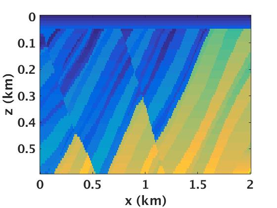
To provide further evidence of the computational and memory savings due to probing, we retrieve the matrix \({\mathbf{\widetilde{R}}}\) from a central part of the Marmousi model (Figure 1). We choose a small section so we can form \({\mathbf{\widetilde{R}}}\) explicitly for comparison. Still this toy section does contain strong lateral variations and dipping reflectors. We use a fixed-spread acquisition configuration with a model grid spacing of \(5\) m, \(401\) co-located sources and receivers with \(10\) m spacing. We only perform comparison for a single frequency at \(10\) Hz. The source wavelet is a Ricker wavelet with a peak frequency of \(30\) Hz. The results are displayed in Table 1 where we report the computational time (in seconds) and memory (in MB) required to compute \({\mathbf{\widetilde{R}}}\) at a single point in the subsurface. Although we get the same common-image point gather using the classical approach versus the proposed approach, probing reduces the computational time by a factor of ten and memory requirement by a factor of twenty. This is a first illustration of the computational and memory benefits of probing techniques over classical dense matrix techniques.

	\(\#\) of PDE solves	time (s)	memory (MB)
conventional	\(2N_s\)	190	710
this paper	\(3 N_x\)	15	35

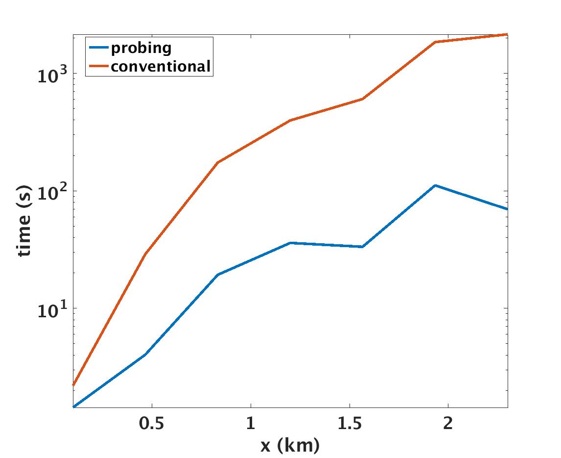
To understand how our approach scales, we also plot a comparison between computational times of probing and the conventional approach as we increase the size of the Marmousi model (Figure 2). This example confirms that our method indeed scales better. We can see that the difference in computational time is substantial with respect to the model size even for this small 2D example. We expect the benefit of our probing technique to be even more pronounced when we switch from 2D to 3D seismic data acquisition where both the size of the model and the number of sources grow drastically.

Target-oriented imaging with probing

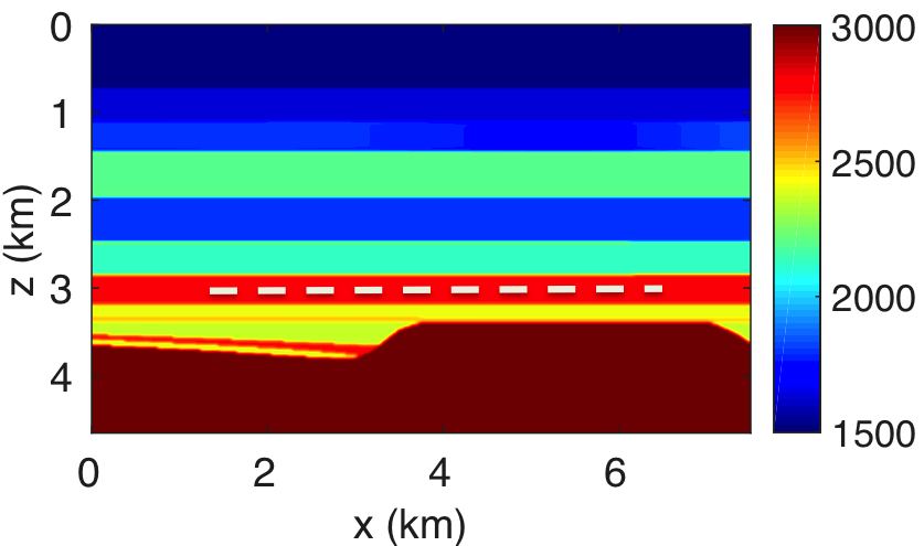
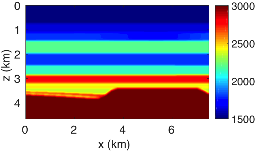
We further demonstrate the advantages of probing for redatuming and target-oriented imaging. To do so, we first consider a simple velocity model consisting of horizontal layers with low-velocity zones and a complex basement structure with a fault (see Figure 3). The aim here is to remove the effect of a low-velocity zone to better image the basement of interest. For this example, the velocity model is \(4.6\,\mathrm{km}\) deep and \(7.5\,\mathrm{km}\) wide, sampled at \(5\,\mathrm{m}\). The synthetic data are computed from \(376\) sources and receivers sampled at \(20\,\mathrm{m}\), respectively. We used the range of frequencies from \(5\) to \(45\,\mathrm{Hz}\) sampled at \(0.25\,\mathrm{Hz}\), where the source-signature is a Ricker wavelet with a central frequency of \(20\) Hz. The subsurface datum \(\partial D_d\) is represented by the dashed white line in Figure 3a. To capture the redatuming data created by the complex basement with fault, we take \(K = 50\) virtual subsurface locations with a sampling interval of \(20\,\mathrm{m}\), which covers the area of interest, and compute the reflection response according to the method outlined above.

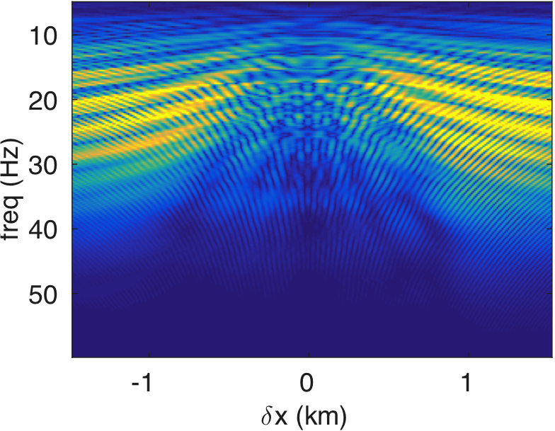
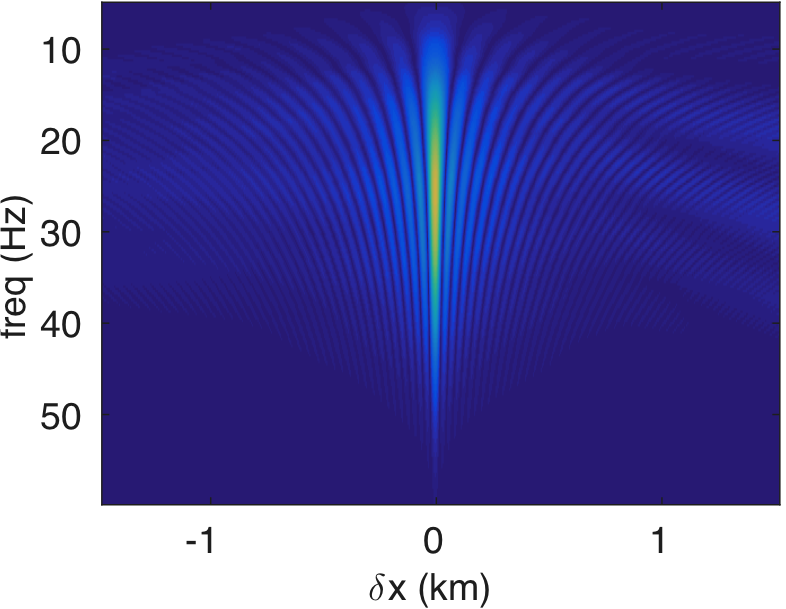
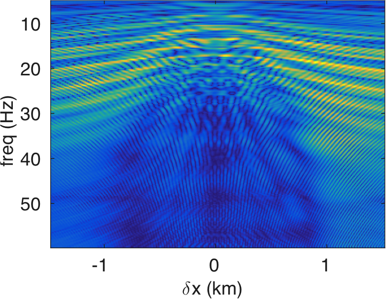
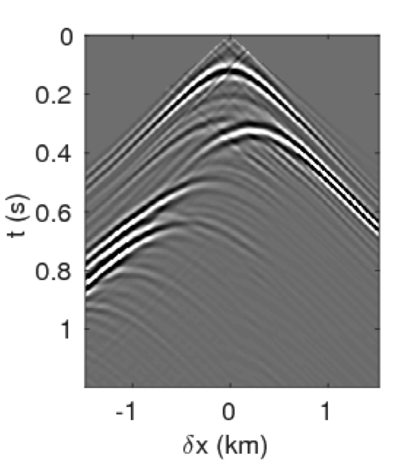
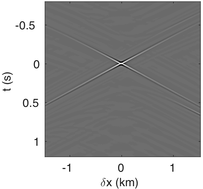
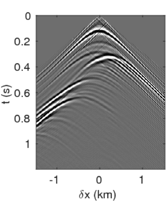
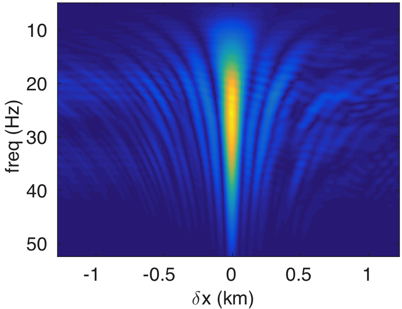
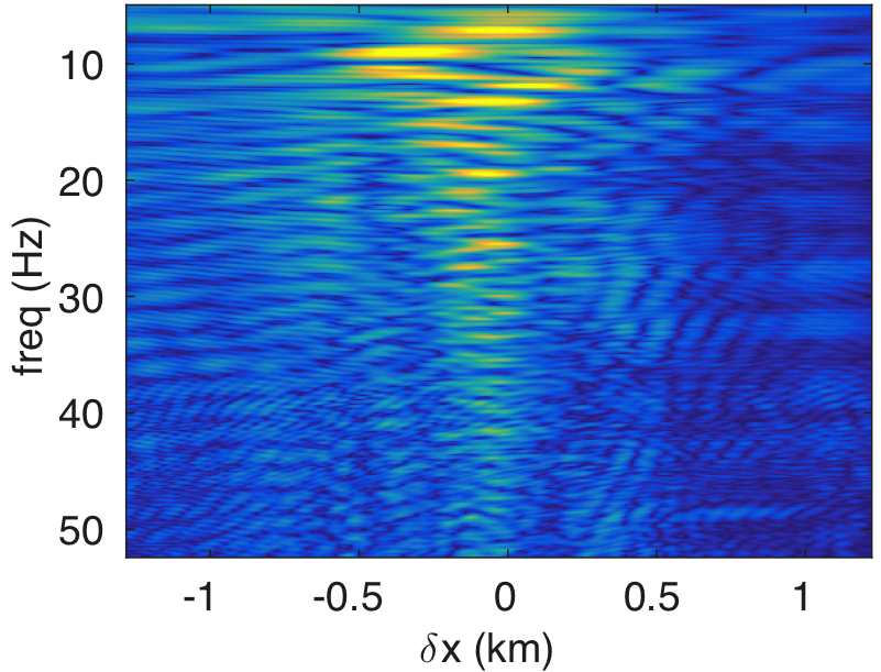
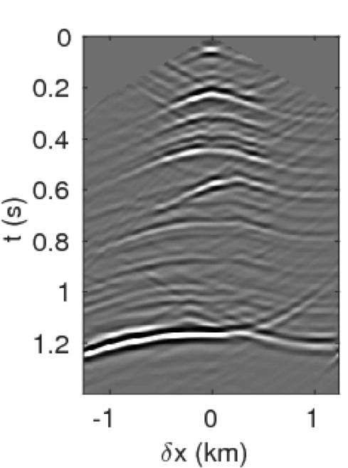
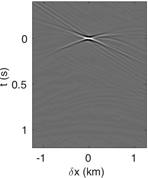
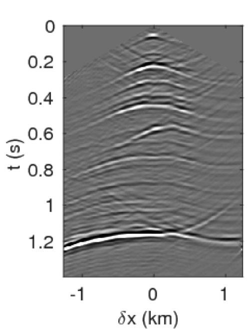
Figures 4a - 4c and 4d - 4f show the frequency-space domain and time-space domain reflection responses at datum point \(x = 3\) and \(z = 2.5\,\mathrm{km}\) before and after source-side blurring correction. To calculate the frequency-space domain reflection response, we solve equation \(\eqref{fin}\) for all the frequencies, followed by restricting it to the subsurface datum \(\partial D_d\), which will results in a reflection matrix \({\mathbf{R}}\) where rows correspond to frequencies and columns correspond to horizontal offset \(\delta x\). For \(K\) probing vectors, \({\mathbf{R}}\) will be a 3D tensor of size \(N_{\delta x} \times K \times N_\omega\). We perform the inverse Fourier-transform along the time-axis to go from frequency-space domain to time-space domain. In Figure 4c, we observe that the energy across the frequency spectrum of \({\mathbf{R}}\) is well distributed compared to the spectrum of \(\mathbf{E}\). This results in a better resolution of reflection events as observed in time-space domain sections in Figure 4f. In this relatively small numerical example, the computation of reflection response by probing is almost three-times faster than its shot-profile counterpart.

The time-domain reverse-time migration images before and after blurring correction are shown in Figures 5a, 5b. We can see that the blurring correction makes the reflectors sharper but creates ringing effects, which is a side effect of MDD. To remove some of these artifacts, Herrmann and Wang (2008) ; van der Neut and Herrmann (2013) proposed to a curvelet-based sparsity promotion approach to perform the MDD, which is more stable with respect to missing data, finite aperture, and bandwidth limitation. We will address this issue in a future paper and concentrate on the computational aspects.

Although probing techniques are an elegant approach to retrieve the reflection response in a computationally feasible manner, this approach only gives us limited access to the full subsurface reflection matrix. Consequently, each new target of interest requires new computations of \(\mathbf{\widetilde{E}}\) and \(\mathbf{\widetilde{\Gamma}}\). This can become an expensive procedure when we are interested in multiple targets especially when we are dealing with large-scale 3D problems. To address this issue, we propose to exploit the low-rank structure of full subsurface extended image volumes themselves. In this approach, the idea is to factorize the full subsurface image volumes, i.e., \(\mathbf{\widetilde{E}}\) and \(\mathbf{\widetilde{\Gamma}}\). Given this factorized form, we can again use probing with \(\mathbf{W}\) to extract the columns of interest from \(\mathbf{\widetilde{E}}\) and \(\mathbf{\widetilde{\Gamma}}\). Of course, this approach is only viable if we manage to keep the number of probing vectors required by the low-rank factorization process small compared to the number of sources.

Low-rank factorization of image volumes — a randomized SVD approach

As we mentioned before, a monochromatic full subsurface extended image volume is a matrix of size \(N_x \times N_x\), where \(N_x\) is the total number of subsurface grid points. Clearly, this is a very large object, especially in 3D, suggesting a need to exploit possible redundancies living in these volumes. Mathematically, matrices with redundancy of information exhibits a low-rank structure. Following the gist of our probing approach, we analyze the decay of the singular values of these volumes for a realistic complex geological model to see whether these extended image volumes can indeed be factored into a low-rank form. In particular, we are interested in whether these singular values decay fast so that these volumes can be approximated accurately by a rank \(r\) matrix, where \(r\ll N_x\). According to equation \(\eqref{ref3}\), the rank of the monochromatic full subsurface extended image volume is linked to the rank of the data matrix \(\mathbf{D}\) or the source matrix \(\mathbf{Q}\) and is equal to \(N_s\) where \(N_s \ll N_x\). While \(\mathbf{Q}\) is full rank when using spatially impulsive monopole source, in which case it corresponds to the identity matrix, the singular values of \(\mathbf{D}\) typically decay quickly especially at the low to mid frequencies. This property allows us to factorize the extended image volume into a \(r\)-rank matrix with \(r\ll N_s\) for the lower frequencies. For higher frequencies, the singular values of \(\mathbf{D}\) decay less rapidly, which eventually leads to an upper bound smaller or equal to \(N_s\) for the image volumes.

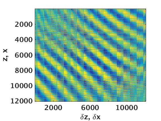
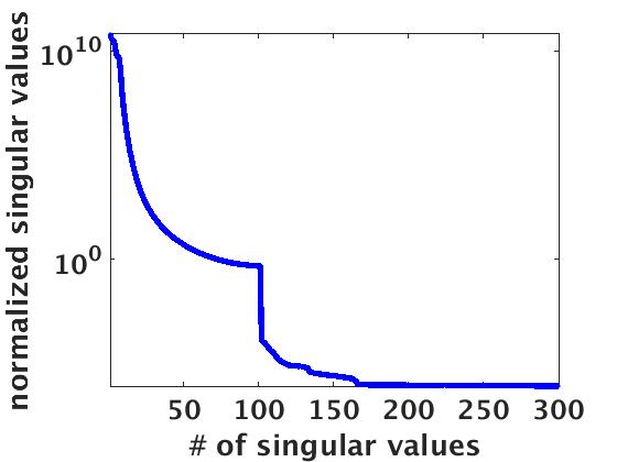
To illustrate that image volumes indeed permit low-rank factorizations at lower frequencies, we again consider a small but geologically complex subset of the Marmousi model, which consists of strongly dipping reflectors with strong lateral velocity variations (Figure 6a). We work with this small subset so that we can compare the time and storage requirements to an explicitly formed full subsurface extended image volume. Even for these complex velocity models, we observe in Figure 6c a fast decay for the extended image at \(5\,\mathrm{Hz}\) depicted in Figure 6b. This observation is crucial for our approach because it demonstrates that even for complex velocity models full subsurface extended image volumes exhibit a low-rank structure, which allows us to approximate the original image volume at \(50\,\mathrm{dB}\) by only using the top ten singular values.

From the example of Figure 6, we can clearly see that even for complex geological structures, the full subsurface extended image volume exhibits a low-rank behavior, a property we can exploit to compress the full subsurface extended image volume in its factorized form. We do this by only computing the top \(r\) singular vectors of \(\mathbf{E}\). While such an approach has obvious benefits some important limitations of the proposed approach remain, namely (i) we need to solve \(2N_s\) PDE’s to form and store full subsurface image volume, which is computationally prohibitively expensive, and (ii) the cost of singular value decomposition (SVD) of a dense explicit full subsurface image volume is of the order of \(\mathcal{O}(N_x^3)\) using naive SVD algorithms (Holmes et al. (2007)).

To circumvent these prohibitive computational costs, we propose to use randomized SVDs (Halko et al., 2011) to compute our low-rank approximation of full subsurface extended image volumes. Randomized SVDs (see Algorithm 2) derive from probings and have a computational time of \(O(N_x^2 \times r)\), which can lead to significant gains if \(r\) is small. As we can see from Algorithm 2, the computational costs of randomized SVDs are dominated by the costs of evaluating PDEs in lines 1 and 3. Aside from these expensive PDE solves, Algorithm 2 also involves carrying out a QR factorization and an SVD. However, the costs associated with these operations are small because they involved operations on probed quantities—i.e., \(\mathbf{Y} \in \mathbb{C}^{N_x \times r}\) and \(\mathbf{Z} \in \mathbb{C}^{r \times N_x}\) are both tall and thin matrices that require a total of only \(4r\) (cf. \(2\times N_s\) PDE solves for conventional methods that loop over shots) PDE solves to evaluate. In addition to obvious computational gains, our SVD-based matrix factorization also allows us to store and form (through actions) extended image volumes while retaining most of the energy in \(\mathbf{E}\).

1. Inputs – source matrix \(\mathbf{Q}\), data matrix \(\mathbf{D}\), and \((N_x \times r)\) Gaussian random probing matrix \(\mathbf{X}\)  
2. Outputs – singular value decomposition of extended image volumes \(\mathbf{G}\), \(\mathbf{S}\), and \(\mathbf{F}\)
3. \(\widetilde{\mathbf{Y}} = \mathbf{E} \mathbf{X}\) (matrix-free operation like in Algorithm 1), where \(\mathbf{E}\) is a function of \(\mathbf{Q}\) and \(\mathbf{D}\)
4. \([\widetilde{\mathbf{B}},\widetilde{{\mathbf{C}}}] = \text{qr}(\widetilde{\mathbf{Y}})\)
5. \(\widetilde{\mathbf{Z}} = \widetilde{\mathbf{B}}^* \mathbf{E}\) (Transpose of matrix-free operation like Algorithm 1)
6. \([{\mathbf{G}},\mathbf{S},{\mathbf{F}}] = \text{svd}(\widetilde{\mathbf{Z}})\) (\(\widetilde{\mathbf{Z}} \in \mathbb{C}^{r \times N_x}\) is a small matrix)
7. \({\mathbf{G}} \gets \widetilde{\mathbf{B}}{\mathbf{G}}\)

Note that, we observed the same low-rank behavior for the matrix \(\mathbf{\Gamma}\), hence, we also exploit its low-rank structure in the multi-domain experimental section using the randomized SVD algorithm, where we replaced \(\mathbf{E}\) with \(\mathbf{\Gamma}\) in Algorithm 2 . Given the low-rank matrix factorization form for \(\mathbf{E}\) and \(\mathbf{\Gamma}\), i.e., \(\mathbf{E} \approx {\mathbf{G}}_1 \mathbf{S}_1 {{\mathbf{F}}_1^{*}}, \) and \(\mathbf{\Gamma} \approx {\mathbf{G}}_2 \mathbf{S}_2 {{\mathbf{F}}_2^{*}}\), we can extract any column from \(\mathbf{E}\) and \(\mathbf{\Gamma}\) via probing with basis vectors \({\mathbf{w}}_j = [0, \ldots, 0, 1, 0,\ldots, 0]\), i.e., \(\mathbf{\widetilde{E}} \approx {{\mathbf{G}}}_1 {\mathbf{S}}_1 {{{\mathbf{F}}}_1^{*}}{\bf{w}}_j\) and \(\mathbf{\widetilde{\Gamma}} \approx {{\mathbf{G}}}_2 {\mathbf{S}}_2 {{{\mathbf{F}}}_2^{*}}{\bf{w}}_j\). As mentioned before, here, \({\bf{w}}_j\) corresponds to the grid location of the point scatterer at datum \(\partial D_d\). Finally, our randomized SVD-based multi-domain target-oriented imaging consists of the following main steps: (i) compute the low-rank factorization form of \(\mathbf{E}\) and \(\mathbf{\Gamma}\) using Algorithm 2; (ii) extract columns from \(\mathbf{E}\) and \(\mathbf{\Gamma}\) corresponding to the grid location of the point scatterer at datum \(\partial D_d\); (iii) perform multidimensional deconvolution to get reflection response matrix \({\mathbf{R}}\).

Remark: Randomized SVDs, derived from actions of \(\mathbf{E}\) and \(\mathbf{E}^{\ast}\) are not the only option to factorize \(\mathbf{E}\) using the top \(r\) singular vectors. Krylov methods (Larsen (1998); Liu et al. (2013)) can accomplish the same decomposition. However, randomized SVDs based methods have at least two main advantages over Krylov based methods. First, the matrix-vector multiplication to form \(\widetilde{\mathbf{Y}}\) and \(\widetilde{\mathbf{Z}}\) can be performed in parallel. This observation allows us to take full advantage of parallel and distributed machines, especially in cloud-computing environment. Second, randomized SVDs have enabled the development of highly efficient single-pass matrix factorization algorithms (Martinsson, 2016), where the communication cost is low and we never have to stored the matrices explicitly. For detailed comparison of Krylov methods and randomized SVDs, we refer the interested readers to Halko et al. (2011) ; Martinsson (2016) . Because of the above mentioned reasons, we opt for randomized SVDs in this work.

Target-oriented imaging using randomized SVD

To demonstrate the computational and memory benefits of our approach with randomized SVD over the classical approach to approximate full subsurface image volume, we compare computation times and memory use for a subset of the Marmousi model, sampled at \(10\,\mathrm{m}\). The simulated data consists of \(301\) coincident sources and receivers both sampled at \(20\,\mathrm{m}\). As before, we use a Ricker wavelet with a central frequency of \(30\,\mathrm{Hz}\). To show the benefits over the full bandwidth of the underlying signal, we compute monochromatic full subsurface image volumes for eight frequencies ranging from \(5\) to \(50\,\mathrm{Hz}\).

As we mentioned before, the rank of the extended image volume is indeed intrinsically linked to the data matrix from Formula \(\eqref{prob}\), hence, we compute \(r\) by looking at the singular values of data. Although, we get an approximation of rank \(r\) using data matrix, this is not the optimal way of choosing the rank since the singular values decay of the data matrix is slower than the corresponding decay of the image volume. By keeping only the number of singular values higher than 10% of the largest one, we obtain the approximated rank values for each frequency. We then use this estimated rank value for each frequency and solve Algorithm 2 to compute the low-rank factorization form of the full subsurface extended image volumes. For comparison, we also form the full subsurface extended image volume using the classical approach. As summarize in Table 2, randomized SVD based approach reduces the computational time of forming the full subsurface image volume by a factor of approximately twenty-five. This major improvement in computational time is due to a reduction in the number of PDE solve (\(2r\ll 2 N_s\)). Moreover, we only need to store \({\mathbf{G}},\mathbf{S}\) and \({\mathbf{F}}\) matrices, thus, the storage of the extended image volumes using randomized SVD is \(r \times (2N_x +1) \) (Algorithm 2). Even though the estimated rank increases with the frequency in Table 2, it is still much smaller than the number of shots needed to form the full extended image volume. Finally, we compare the low-rank approximation of the extended image volume with the full extended image volume by computing the signal-to-noise ratio that is above \(20\,\mathrm{dB}\) for all eight frequencies. Thus the approximation of full subsurface extended image volume using randomized SVD is satisfactory.

frequency (\(\mathrm{Hz}\))	real rank	full time (\(\mathrm{s}\))	estimated rank	reduced time (\(\mathrm{s}\))	SNR (\(\mathrm{dB}\))	memory ratio
5	301	490	7	11	29	43
10	301	490	8	11	24	38
15	301	490	10	12	21	30
20	301	490	11	12	20	28
25	301	490	13	13	22	24
30	301	490	16	15	22	19
40	301	490	20	17	22	15
50	301	490	25	21	20	12

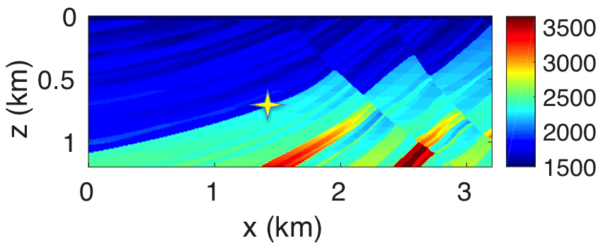
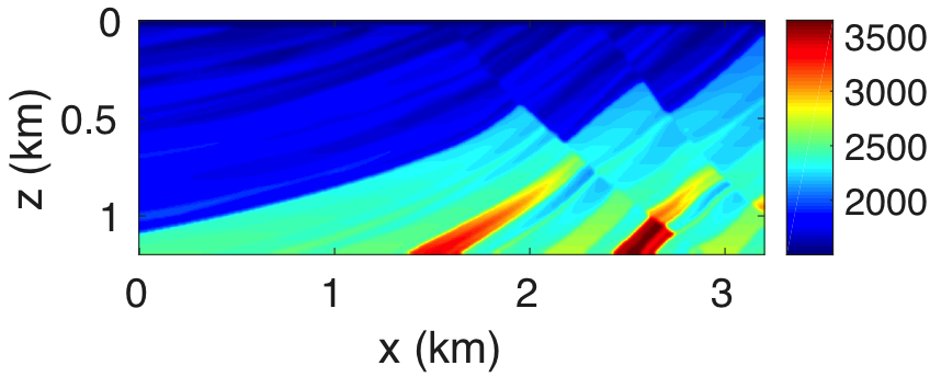
Finally, we demonstrate our approach in a more realistic setting, namely a subsection of the Sigsbee2A model (The SMAART JV, 2001), which contains complex sedimentary basins interspersed with a high-contrast and high-velocity salt body. The velocity model depicted in Figure 7 is \(6\,\mathrm{km}\) deep and \(7.5\,\mathrm{km}\) wide and sampled at \(5\,\mathrm{m}\). In total, we acquire \(1502\) coincident sources and receivers sampled at \(5\,\mathrm{m}\). As before, we use a Ricker wavelet as a source function with a central frequency of \(30\,\mathrm{Hz}\). To compute the reflection response matrix \({\mathbf{R}}\), we use frequencies from \(5\) to \(55\,\mathrm{Hz}\) with a sampling interval of \(0.125\,\mathrm{m}\). We perform the target-oriented imaging at the subsurface datums \(\partial D_d\) represented by the black line in Figure 7a.

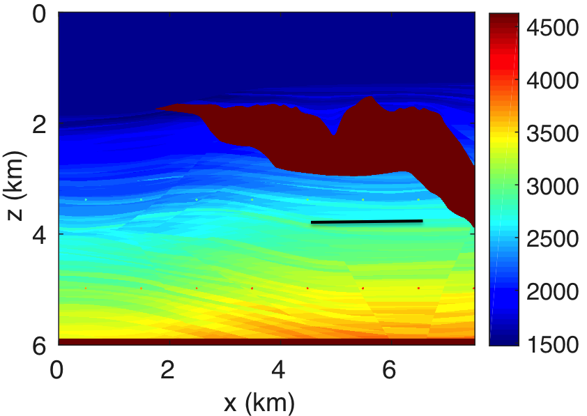
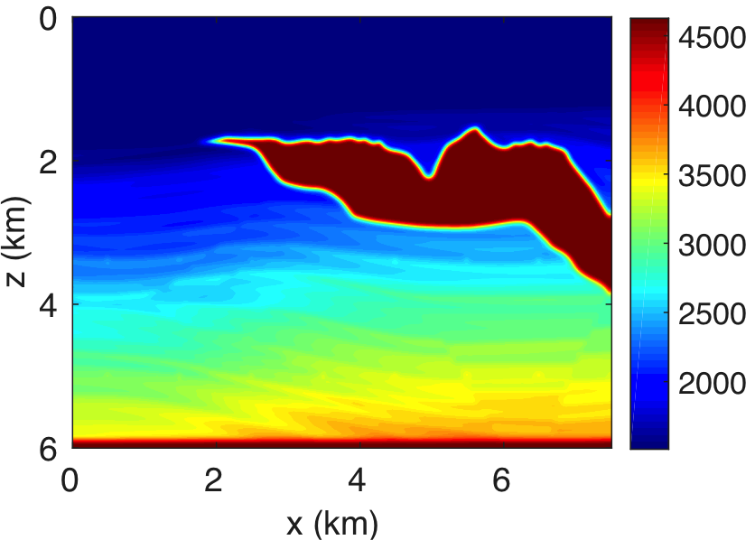
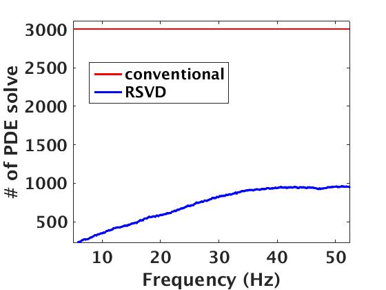
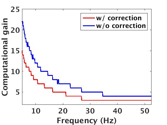
Figure 8a shows the estimated rank values as a function of the frequencies, which we compute by keeping the number of singular values of data higher than 10% of the largest one. We use these rank values in our randomized SVD algorithm 2 to approximately factorize \(\mathbf{E}\) and \(\mathbf{\Gamma}\). Figure 8b displays the total number of PDE’s solves needed to compute this approximation as a function of increasing frequency and compares it to the conventional method, which requires \(N_s\) PDE solves on top of computing cross-correlations between the forward and adjoint wavefield prior to summing over time. From this approach, it is evident that our randomized SVD method is computationally efficient both in its required number of PDE solves (\(r\) versus \(N_s\)) and cross-correlation costs (cross correlations in data versus model space). However, it is not unexpected that the numerical efficiency decreases as we move to higher frequencies. Monochromatic seismic data exhibit low-rank structure only at the low- and intermediate frequencies, but less so at the high-frequencies, i.e., above 60 Hz. This behavior can be explained because wavefields become increasingly oscillatory at high frequencies. In addition to these computational gains, we save a factor of \(\approx\) fifteen in memory usage, while forming the full subsurface extended image volumes using the proposed factorization based approach. Apart from memory savings, Figure 9 shows the gain in the computational time to form full subsurface extended image volume using the proposed randomized SVD approach compared to the shot-profile based extended imaging approach. The memory storage and the computational efficiency make the randomized SVD based approach a true enabler for performing the target-oriented imaging for large-scale 3D acquisition.

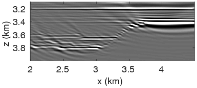
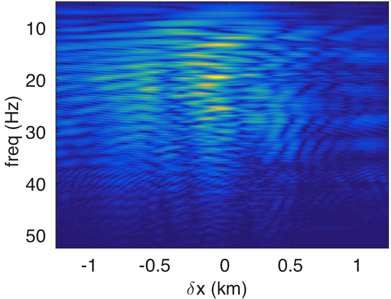
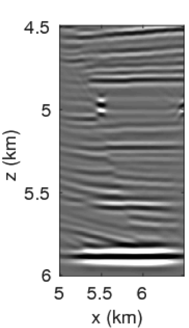
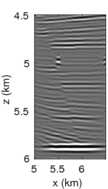
Figures 10a - 10c and 10d - 10f display the frequency-space domain and time-space domain data before and after source-side blurring correction, for the subsurface datums \(\partial D_d\) represented by the black line. We again perform the inverse Fourier transform along the frequency axis to go from frequency-space domain to time-space domain. In Figure 10c, we can observe that energy is distributed evenly along lower and higher end of the frequency spectrum of \({\mathbf{R}}\) compared to the spectrum of \(\mathbf{E}\) in Figure 10a. The well balanced energy distribution along the spectrum results in more sharper (high-resolution) reflection events as evident in time-domain sections (cf. Figures 10d and 10f). Figures 11a and 11b show the reverse-time migration images before and after our blurring correction. From these Figures, we see that the increase in the energy distribution across the frequencies after the blurring correction improves the resolution of reflectors.

Discussion

The main objective of target-oriented wave-equation based imaging is to reduce demand for computational and storage resources to create images in localized areas. While many of the proposed approaches to redatuming make claims to this effect, the majority of the approaches still require expensive loops over shots that involve simulations of forward and adjoint wavefields over the full domain. In most cases, reported gains can be attributed to the use of target-based imaging conditions over the targeted domain of interest, which leads to savings in compute and storage of the wavefields.

By using techniques from randomized linear algebra, we avoid the expensive loops over shots, explicit storage of the forward and adjoint wavefields, and computations of cross-correlations that involve these wavefields. Instead, we work with low-rank factorizations of full-subsurface image volumes. We reap information needed to form these factorizations via actions of extended image volumes on random probing vectors that act as subsurface simultaneous sources. By using the wave equations themselves to carry out the heavy lifting—e.g, we avoid computing the cross correlations, we achieve significant computational and storage gains as long as we can approximate these image volumes by a low-rank matrix. In that case, the cost of our redatuming scheme is dominated by the rank of the factorization instead of by the main loop over shots while storage of and operations on full wavefields are avoided. As a result, we end up with a computationally feasible and scalable scheme that by virtue of the low-rank singular-value decomposition also allows us to cheaply apply the deconvolution imaging condition.

We verified the viability of our approach in 2D for monochromatic subsurface-offset volumes, which as all extended full-subsurface image volumes, are quadratic in the image size making it impossible to form them explicitly except for the smaller 2D toy problems. Experimentally, we found that an order of magnitude reduction in memory usage and computation time is achievable for the low to mid frequencies where image volumes can well be approximated by a low-rank matrix. In that regime, our method scales to 3D where even bigger computational gains are to be expected as we reported in van Leeuwen et al. (2015). In that case, we could never hope to form the image volumes explicitly so we have to completely rely on our approach based on randomized probing where the cost per probing vector corresponds to only two wave-equation solves. As a result, we gain significantly if the extended image volumes can well be approximated in low-rank form since the costs will scale with this rank.

While we argue that our approach beats conventional approaches, as long as the rank is smaller than the number of shots, we make this claim for the low- to mid-range frequencies where extended image volumes are indeed low rank. For the higher frequencies, we may have to exploit other approaches that include exploiting the low-rank off-diagonal structure of image volumes by hierarchical semi-separable representation (HSS, Chandrasekaran et al. (2006), Lin et al. (2011), Jumah and Herrmann (2014)). Another option would be to use recent work by C. Musco and Musco (2015) on block Krylov methods. In either case, the presented approach has the advantage that the probing can be done in parallel and involves significantly fewer resources because we only need to loop over the rank instead of over shots.

Conclusions

The main premise of wave-equation based redatuming, also known as target-oriented imaging, is that it is computationally efficient. Even though many elegant solutions to target-oriented imaging exist, their computational costs often scale linearly with the number of shots and exponentially with the size of the full model. By using probing techniques from randomized linear algebra, we mitigate these costs by representing image volumes in low-rank factored form. By construction, image volumes can be considered as redatumed data after restriction to a particular datum. The low-rank factorization gives us access to this restriction without having to form, work with or loop over all shots.

Our approach is based on a “double two-way wave equation”, which is an object we can probe at the costs of two wave-equation solves for each probing vector. These probings give us access via the randomized singular-value factorization to redatumed data without the need to loop over shots, which can lead to major computational gains if the rank of the factorization is smaller than the number of shots. Since monochromatic full subsurface extended image volumes indeed exhibit a low-rank structure for low-to-mid range frequencies this leads to a viable approach that leads to significant reductions in computational costs. Rather than being dominated by the number of shots in the survey, our costs are proportional to the rank of the factorization, which is small as long as we do not work at too high frequencies. Experimental results for these low-to-mid range frequencies on synthetic 2D models demonstrate that the proposed low-rank factorization based approach is \(\approx\) twenty-five times faster in time and more than fifteen times cheaper in memory storage compared to the conventional shot-profile approach. We further illustrate experimentally using 2D Sigsbee model that the target-oriented images using low-rank factorization based reflection response can be computed with little to no compromise in accuracy compared to the standard shot-profile approaches.

Acknowledgements

R.K. would like to thank Schlumberger Gould Research Centre, Cambridge, UK, for the internship opportunity, where this project took initial shape. This work was financially supported in part by the Natural Sciences and Engineering Research Council of Canada Collaborative Research and Development Grant DNOISE II (CDRP J 375142-08). This research was carried out as part of the SINBAD II project with the support of the member organizations of the SINBAD Consortium. The authors wish to acknowledge the SENAI CIMATEC Supercomputing Centre for Industrial Innovation, with support from BG Brazil and the Brazilian Authority for Oil, Gas and Biofuels (ANP), for the provision and operation of computational facilities and the commitment to invest in Research and Development. Finally, M.G. would like to thanks the Swiss National Science Foundation (Grant no. P300P2-167681) for financial support.