Solving multiphysics-based inverse problems with learned surrogates and constraints

![]()

Affiliation: Georgia Institute of Technology
Address: 756 West Peachtree Street NW, Atlanta, Georgia, USA 30308
Emails:
Ziyi Yin (corresponding author): ziyi.yin@gatech.edu
Rafael Orozco: rorozco@gatech.edu
Mathias Louboutin: mlouboutin3@gatech.edu
Felix J. Herrmann: felix.herrmann@gatech.edu
Abstract
Solving multiphysics-based inverse problems for geological carbon storage monitoring can be challenging when multimodal time-lapse data are expensive to collect and costly to simulate numerically. We overcome these challenges by combining computationally cheap learned surrogates with learned constraints. Not only does this combination lead to vastly improved inversions for the important fluid-flow property, permeability, it also provides a natural platform for inverting multimodal data including well measurements and active-source time-lapse seismic data. By adding a learned constraint, we arrive at a computationally feasible inversion approach that remains accurate. This is accomplished by including a trained deep neural network, known as a normalizing flow, which forces the model iterates to remain in-distribution, thereby safeguarding the accuracy of trained Fourier neural operators that act as surrogates for the computationally expensive multiphase flow simulations involving partial differential equation solves. By means of carefully selected experiments, centered around the problem of geological carbon storage, we demonstrate the efficacy of the proposed constrained optimization method on two different data modalities, namely time-lapse well and time-lapse seismic data. While permeability inversions from both these two modalities have their pluses and minuses, their joint inversion benefits from either, yielding valuable superior permeability inversions and CO2 plume predictions near, and far away, from the monitoring wells.
Keywords: Fourier neural operators, normalizing flows, multiphysics, deep learning, learned surrogates, learned constraints, inverse problems
Introduction
In this paper, we introduce a novel learned inversion algorithm designed to address inverse problems based on partial differential equations (PDEs). These problems can be represented using the following general form:
\[ \mathbf{d} = \mathcal{H}\circ\mathcal{S}(\mathbf{K}) + \boldsymbol \epsilon. \tag{1}\]
In this expression, the nonlinear operator \(\mathcal{S}\) represents the solution operator of a nonlinear parametric PDE mapping the coefficients \(\mathbf{K}\) to the solution. Given numerical solutions of the PDE, partially observed data, collected in the vector \(\mathbf{d}\), are modeled by compounding the solution operator with the measurement operator, \(\mathcal{H}\), followed by adding the noise term \(\boldsymbol{\epsilon}\) with noise level of \(\sigma\)—i.e., \(\boldsymbol{\epsilon}\sim \mathcal{N}(\mathbf{0}, \sigma^2 \mathbf{I})\). This problem is quite general and pertinent to various physical applications, including geophysical exploration (Tarantola 1984, 2005), medical imaging (Arridge 1999), and experimental design (Alexanderian 2021).
Without loss of generality, we focus on time-lapse seismic monitoring of geological carbon storage (GCS), which involves underground storage of supercritical CO2 captured from the atmosphere or from industrial smoke stacks (Furre et al. 2017). We consider GCS in saline aquifers, which involves multiphase flow physics where CO2 replaces brine in the porous rocks (Nordbotten and Celia 2011). In this context, the PDE solution operator, \(\mathcal{S}\), serves as the multiphase flow simulator, which takes the gridded spatially varying permeability in the reservoir, \(\mathbf{K}\), as input and produces \(n_t\) time-varying CO2 saturation snapshots, \(\mathbf{c}=[\mathbf{c}_1, \mathbf{c}_2, \cdots,\mathbf{c}_{n_t}]\), as output. The governing equations for the multiphase flow involve Darcy’s and the mass conservation law. Detailed information on the governing equations, initial and boundary conditions, and numerical solution schemes can be found in (Rasmussen et al. 2021) and the references therein. To ensure safety, conformance, and containment of GCS projects, various kinds of time-lapse data are collected to monitor CO2 plumes. These different data modalities include measurements in wells (Freifeld et al. 2009; Nogues, Nordbotten, and Celia 2011), and the collection of gravity (Nooner et al. 2007; Alnes et al. 2011), electromagnetic (Carcione et al. 2012; Zhdanov et al. 2013), and seismic time-lapse data (Arts et al. 2004; Lumley 2010; Yin et al. 2023) that can be used to follow the plume and invert for reservoir properties such as the permeability, \(\mathbf{K}\). The latter is the property of interest in this exposition.
Overall, solving for the reservoir model parameter, \(\mathbf{K}\), poses significant challenges for two primary reasons:
the forward modeling operator, \(\mathcal{H}\circ\mathcal{S}\), can be ill-posed, resulting in multiple model parameters that fit the observed data equally well. This necessitates the use of regularizers (Golub, Hansen, and O’Leary 1999; Tarantola 2005) in the form of penalties or constraints (Peters, Smithyman, and Herrmann 2019).
The PDE modeling operator \(\mathcal{S}\), and the sensitivity calculations with respect to the model parameters can be computationally expensive for large-scale problems, limiting the efficacy of iterative methods such as gradient-based (D. C. Liu and Nocedal 1989) or Markov chain Monte Carlo (Cowles and Carlin 1996) methods.
To overcome the second challenge, numerous attempts have been made to replace computationally expensive PDE solves with more affordable approximate alternatives (Razavi, Tolson, and Burn 2012; Asher et al. 2015), which include the use of radial basis functions to learn the complex models from few sample points (Powell 1985) or reduced-order modeling where the dimension of the model space is reduced (Schilders, Van der Vorst, and Rommes 2008; K. Lu et al. 2019). More recently, various deep learning techniques have emerged as cheap alternatives to numerical PDE solves (L. Lu, Jin, and Karniadakis 2019; Pestourie et al. 2020; Qian et al. 2020; Karniadakis et al. 2021; Kovachki et al. 2021; Rahman, Ross, and Azizzadenesheli 2022; Hijazi, Freitag, and Landwehr 2023). After incurring initial training costs, these neural operators lead to vastly improved computation of PDE solves. Data-driven methods have also been used successfully to learn coarse-to-fine grid mappings of PDEs solves. Because of their advertised performance on approximating solution operators of the multiphase flow in porous media (G. Wen et al. 2022, 2023; Grady et al. 2023; Philipp A. Witte, Redmond, et al. 2022; Philipp A. Witte, Hewett, et al. 2022; Philipp A. Witte et al. 2023), we will consider Fourier neural operators (FNOs, Z. Li et al. 2020; Kovachki, Lanthaler, and Mishra 2021) in this work even though alternative choices can be made. Once trained, FNOs produce approximate PDE solutions orders of magnitude faster than traditional solvers (Z. Li et al. 2020, 2021; Grady et al. 2023; De Hoop et al. 2022). In addition, Yin et al. (2022), Louboutin et al. (2022) and Louboutin, Yin, et al. (2023) demonstrated that trained FNOs can replace PDE solution operators during inversion. This latest development is especially beneficial to applications such as GCS where trained FNOs can be used in lieu of numerically costly flow simulators (Lie 2019; Rasmussen et al. 2021; Gross and Mazuyer 2021). However, despite their promising results, unconstrained inversion formulations offer little to no guarantees that the model iterates remain within the statistical distribution on which the FNO was trained initially during inversion. As a consequence, FNOs may no longer produce accurate fluid-flow simulations throughout the iterations, which can lead to erroneous inversion results when the errors become too large, possibly rendering surrogate modeling by FNOs ineffective. To avoid this situation, we propose a constrained formulation where a trained normalizing flow (NF, Rezende and Mohamed (2015)) is included as a learned constraint. This added constraint guarantees that the model iterates remain within the desired statistical distribution. Because our approach safeguards the FNO’s accuracy, it allows FNOs to act as reliable low-cost neural surrogates replacing costly fluid-flow simulations and gradient calculations that rely on numerically expensive PDE solves during inversion.
The organization of this paper is as follows: First, we introduce FNOs and explore the possibility of replacing the forward modeling operator with a trained FNO surrogate. Next, NFs are introduced. By means of a motivational example, we demonstrate how these learned generative networks control the prediction error of FNOs by ensuring that the model iterates remain in distribution. Based on this motivational example, we propose our novel method for using trained NFs as a learned constraint to guarantee performance of FNO surrogates during inversion. Through four synthetic experiments related to GCS monitoring, the efficacy of our method will be demonstrated.
Fourier neural operators
There is an extensive literature on training deep neural networks to serve as affordable alternatives to computationally expensive numerical simulators (L. Lu, Jin, and Karniadakis 2019; Karniadakis et al. 2021; Kovachki et al. 2021; Kontolati et al. 2023; Benitez et al. 2023). Without loss of generality, we limit ourselves in this exposition to the training of a special class of neural operators known as Fourier neural operators (FNOs). These FNOs are designed to approximate numerical solution operators of the PDE solution operator, \(\mathcal{S}\), by minimizing the following objective: \[ \underset{\boldsymbol{\theta}}{\operatorname{minimize}} \quad \, \frac{1}{N}\sum_{j=1}^{N}\|\mathcal{S}_{\boldsymbol{\theta}}(\mathbf{K}^{(j)})-\mathbf{c}^{(j)}\|_2^2\quad\text{where}\quad\mathbf{c}^{(j)}=\mathcal{S}(\mathbf{K}^{(j)}). \tag{2}\]
Here, \(\mathcal{S}_{\boldsymbol{\theta}}\) denotes the FNO with network weights \({\boldsymbol{\theta}}\). The optimization aims to minimize the \(\ell_2\) misfit between numerically simulated PDE solutions, \(\mathbf{c}^{(j)}\), and solutions approximated by the FNO, across \(N\) training samples (permeability models), \(\{\mathbf{K}^{(j)}\}_{j=1}^N\) compiled by domain experts. Once trained, FNOs can generate approximate PDE solutions for unseen model parameters orders of magnitude faster than numerical simulations (Grady et al. 2023; De Hoop et al. 2022). For model parameters that fall within the distribution used to train, approximation by FNOs are reasonably accurate—i.e., \(\mathcal{S}_{\boldsymbol\theta^\ast}(\mathbf{K})\approx\mathcal{S}(\mathbf{K})\), with \(\boldsymbol\theta^\ast\) being the minimizer of Equation 2. We refer to the numerical examples section for details calculating these weights. Before studying the impact of applying these surrogates on samples for the permeability that are out of distribution, let us first consider an example where data is inverted using surrogate modeling.
Inversion with learned surrogates
Replacing PDE solutions by approximate solutions yielded by trained FNO surrogates has two main advantages when solving inverse problems. First, as mentioned earlier, FNOs are orders of magnitude faster than numerical PDE solves, which allows for many simulations at negligible costs (Chandra et al. 2020; Lan, Li, and Shahbaba 2022). Second, existing softwate for multiphase flow simulations may not always support computationally efficient calculations of sensitivity, e.g. via adjoint-state calculations (Cao et al. 2003; Plessix 2006; Jansen 2011) of the simulations with respect to their input. In such cases, FNO surrogates are favorable because automatic differentiation on the trained network (Griewank et al. 1989; Louboutin et al. 2022; Yin et al. 2022; Yang et al. 2023; Louboutin, Yin, et al. 2023) readily provides access to gradients with respect to model parameters. As a result, the PDE solver, \(\mathcal{S}\), in Equation 1 can be replaced by trained surrogate, \(\mathcal{S}_{\boldsymbol\theta^\ast}\)—i.e., we have
\[ \underset{\mathbf{K}}{\operatorname{minimize}} \quad \|\mathbf{d} - \mathcal{H}\circ\mathcal{S}_{\boldsymbol\theta^\ast}(\mathbf{K})\|_2^2 \tag{3}\]
where \(\boldsymbol\theta^\ast\) represent the optimized weights minimizing Equation 2. While the above formulation in terms of trained surrogates has been applied successfully during permeability inversion from time-lapse seismic data (D. Li et al. 2020; Yin et al. 2022; Louboutin, Yin, et al. 2023), this type of inversion is only valid as long as the (intermediate) permeabilities remain within distribution during the inversion. Practically, this means two things. First, the data need to be in the range of permeability models that are in distribution. This means that there can not be too much noise neither can the observed data be the result of an out-of-distribution permeability. Second, there are no guarantees that the permeability model iterates remain in distribution during inversion even though some bias of the gradients of the surrogate towards in-distribution permeabilities may be expected. To overcome this challenge, we propose to add a learned constraint to Equation 3 that offers guarantees that the model iterates remain in distribution.
Learned constraints with normalizing flows
As demonstrated by Peters and Herrmann (2017), Esser et al. (2018), Peters, Smithyman, and Herrmann (2019) regularization of non-linear inverse problems, such as full-waveform inversion, with constraints, e.g., total-variation (Esser et al. 2018) or transform-domain sparsity with \(\ell_1\)-norms (X. Li et al. 2012), offers distinct advantages over regularizations based adding these norms as penalties. Even though constraint and penalty formulations are equivalent for linear inverse problems for the appropriate choice of the Lagrange multiplier, minimizing the constraint formulation leads to completely different solution paths compared to adding a penalty term to the data misfit objective (Hennenfent et al. 2008). In the constrained formulation, the model iterates remain at all times within the constraint set while model iterates yielded by the penalty formulation does not offer these guarantees. Peters and Herrmann (2017) demonstrated this importance difference for the non-convex problem of full-waveform inversion. For this problem, it proved essential to work with a homotopy where the intersection of multiple handcrafted constraints (intersection of box and size of total-variation-norm ball constraints) are relaxed slowly during the inversion, so the model iterates remain physically feasible and local minima are avoided.
Motivated by these results, we propose a similar approach but now for “data-driven” learned constraints based on normalizing flows (NFs, Rezende and Mohamed (2015)). NFs are powerful deep generative neural networks capable of learning to generate samples from complex distributions (Dinh, Sohl-Dickstein, and Bengio 2016; Siahkoohi et al. 2023b; Orozco, Louboutin, et al. 2023; Louboutin, Yin, et al. 2023). Designed to be invertible, these NFs require the latent and model spaces to share identical dimensions, which confers several advantages:
unlike variational autoencoders (Kingma and Welling 2013) or generative adversarial networks (GANs, Goodfellow et al. 2014), which both have a lower-dimensional latent space, NFs do not impose any intrinsic dimensionality constraints. This flexibility lets NFs capture model space characteristics across high dimensions (Kobyzev, Prince, and Brubaker 2020). Relevantly, concurrent literature has delved into the intrinsic dimensionality of NFs, indicating the potential to using NFs to generate models with inherently lower dimensions (Horvat and Pfister 2022).
NFs’ inherent invertibility negates the need to store state variables during gradient calculations, enabling memory-efficient training and inversion in large-scale 3D applications, such as in geophysics (Zhang and Curtis 2020, 2021; Siahkoohi et al. 2021, 2023b; Siahkoohi and Herrmann 2021; Zhao, Curtis, and Zhang 2021; Lensink, Peters, and Haber 2022) and ultrasound imaging (Orozco et al. 2021, 2023; Orozco, Louboutin, and Herrmann 2022; Orozco, Louboutin, et al. 2023; Orozco, Siahkoohi, Louboutin, et al. 2023; J. Wen, Ahmad, and Schniter 2023).
because of their invertibility NFs guarantee unique latent codes for all model space samples, including out-of-distribution ones. Therefore, they can still be used to invert for out-of-distribution model parameters, while other methods like GANs may introduce bias (Asim et al. 2020).
Aside from being invertible, NFs are trained to map samples from a target distribution in the physical space to samples from the standard zero-mean Gaussian distribution noise in the latent space. After training is completed, samples from the target distribution are generated by running the NF in reverse on samples in the latent space from the standard Gaussian distribution. Below, we will demonstrate how NFs can be used to guarantee that the permeability remains in distribution during the inversion.
Training normalizing flows
Given samples from the permeability distribution, \(\{\mathbf{K}^{(j)}\}_{j=1}^N\), training NFs entails minimizing the Kullback-Leibler divergence between the base and target distributions (Ardizzone et al. 2018). This involves solving the following variational problem: \[ \underset{\mathbf{w}}{\operatorname{minimize}} \quad \frac{1}{N}\sum_{i=1}^{N} \left(\frac{1}{2}\|\mathcal{G}^{-1}_{\mathbf{w}}(\mathbf{K}_i)\|_2^2-\log\left|\det\mathrm{J}_{\mathcal{G}^{-1}_{\mathbf{w}}}(\mathbf{K}_i)\right|\right). \tag{4}\]
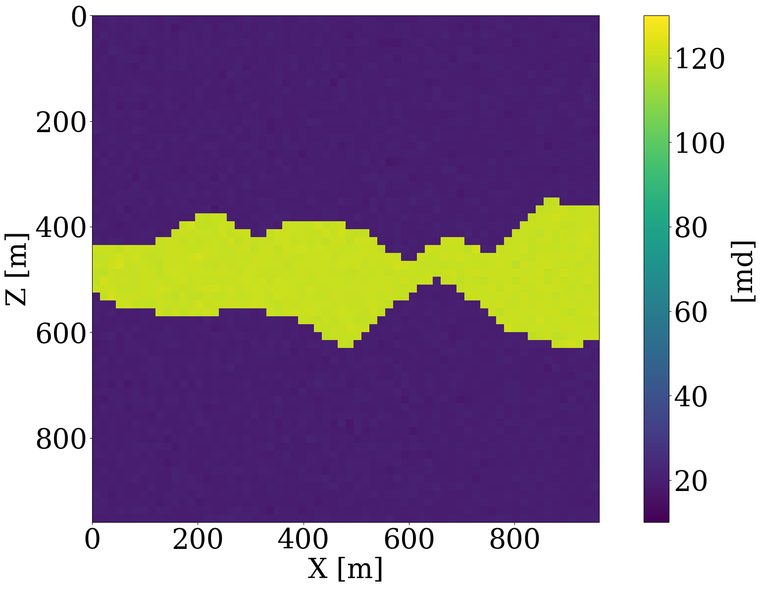
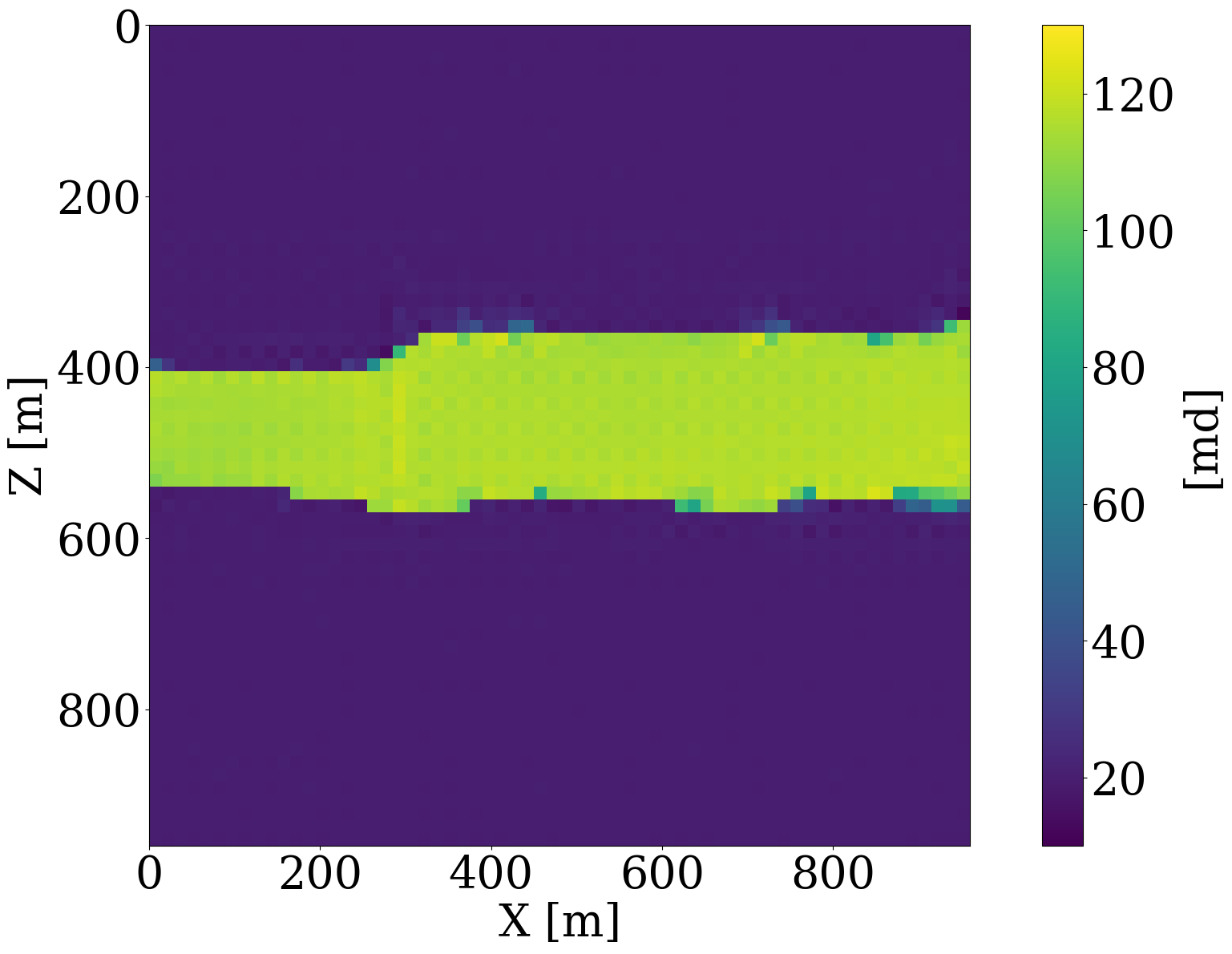
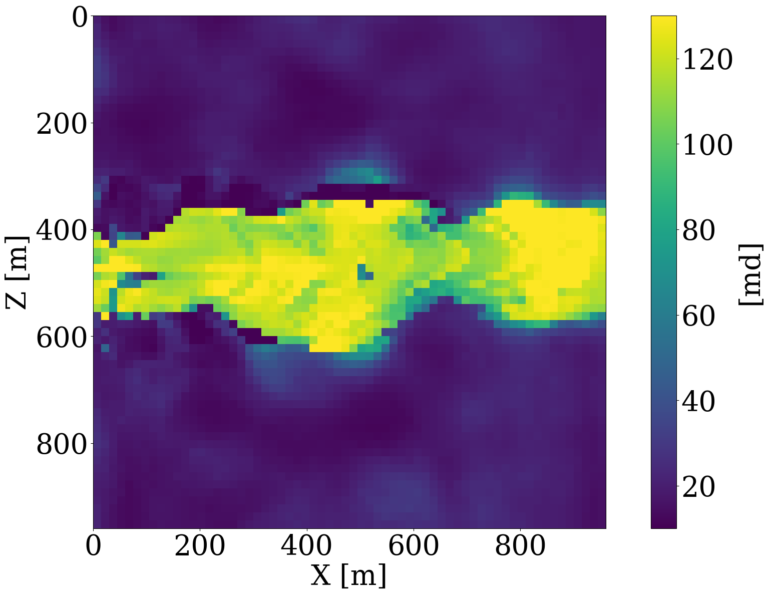
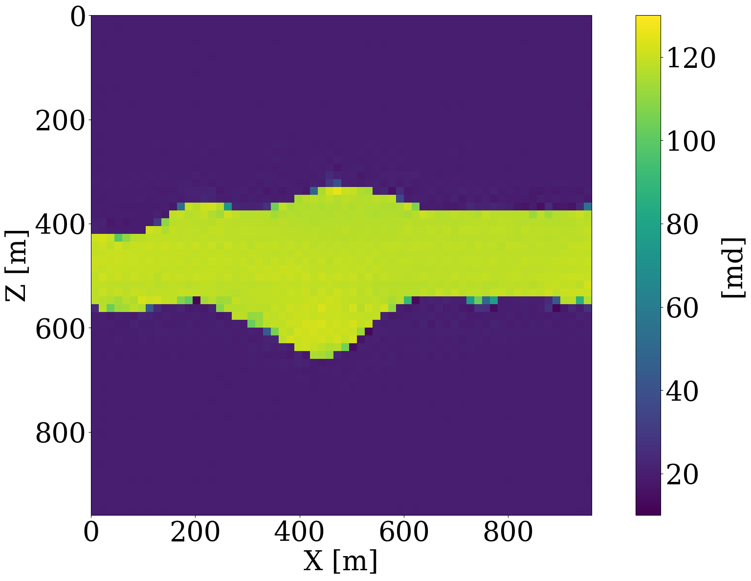
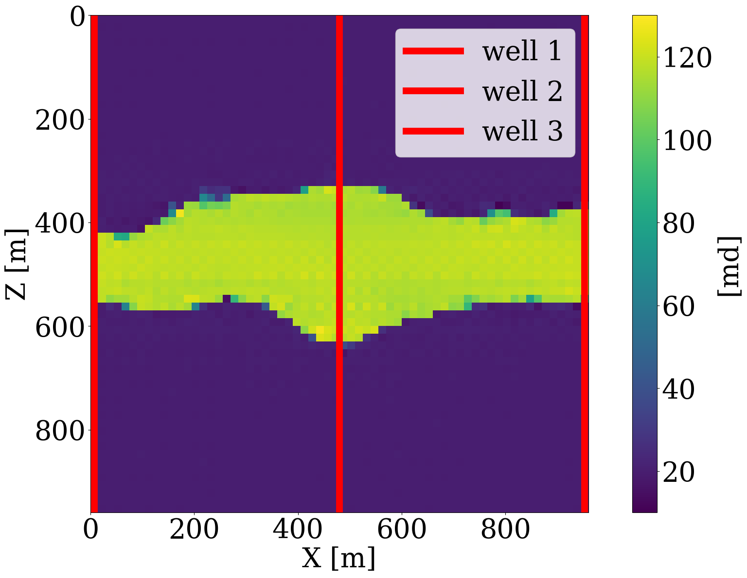
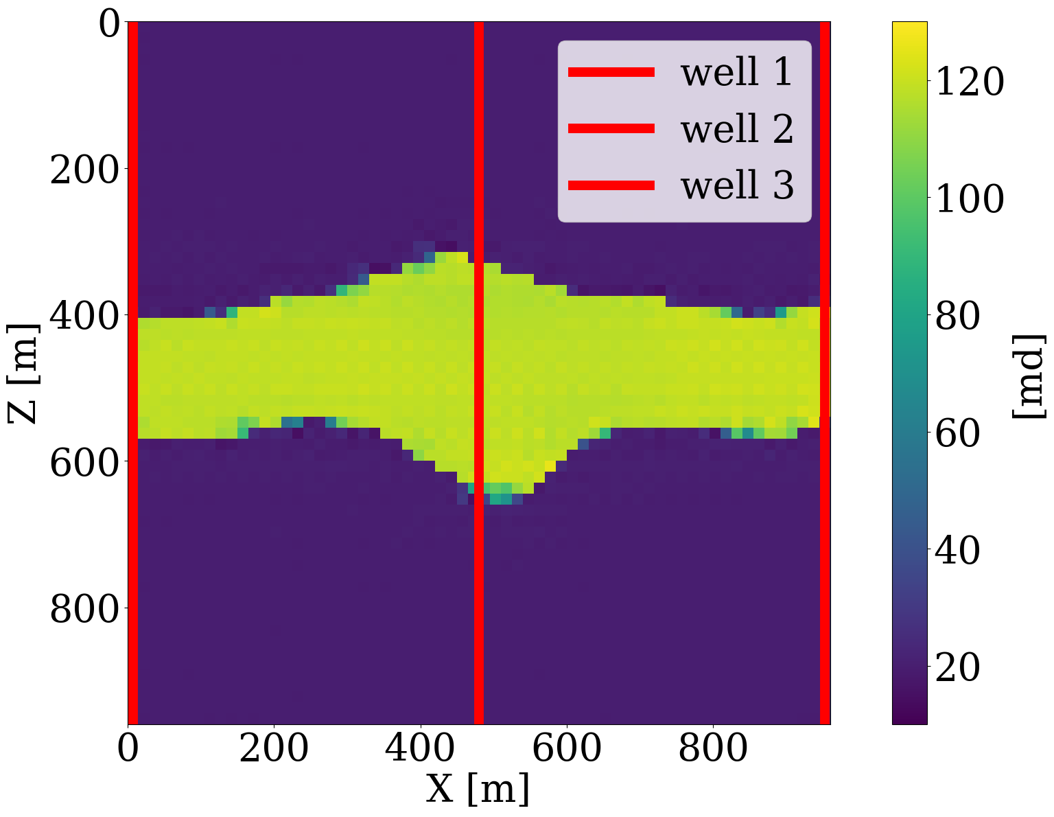
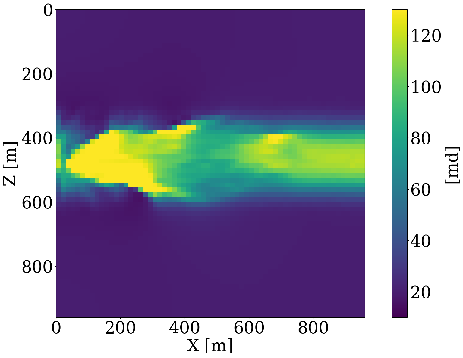
In this optimization problem, \(\mathcal{G}^{-1}_{\mathbf{w}}\) represents the NF, which is parameterized by its network weights \(\mathbf{w}\), while \(\mathrm{J}_{\mathcal{G}^{-1}_{\mathbf{w}}}\) denotes its Jacobian. By minimizing the \(\ell_2\)-norm, the objective imposes a Gaussian distribution on the network’s output and the second \(\log\det\) term prevents trivial solutions, i.e., cases where \(\mathcal{G}^{-1}_{\mathbf{w}}\) produces zeros. To ensure alignment between the permeability distributions, Equation 2 and Equation 4 are trained on the same dataset consisting of 2000 permeability models examples of which are included in Figure 1. Each \(64\times64\) permeability model of consists of a randomly generated highly permeable channels (\(120\,\mathrm{mD}\)) in a low-permeable background of \(20\,\mathrm{mD}\), where \(\,\mathrm{mD}\) denotes millidarcy. Generative examples produced by the trained NF are included in the second row of Figure 1, which confirm the NF’s ability to learn distributions from examples. Aside from generating samples from the learned distribution, trained NFs are also capable of carrying out density calculations, an ability we will exploit below.

Trained normalizing flows as constraints
As we mentioned before, adding constraints to the solution of non-convex optimization problems offers guarantees that model iterates remain within constrained sets. When solving inverse problems with learned surrogates, it is important that model iterates remain “in distribution”, which can be achieved by recasting the optimization problem in Equation 3 into the following constrained form:
\[ \underset{\mathbf{z}}{\operatorname{minimize}} \quad \|\mathbf{d} - \mathcal{H}\circ\mathcal{S}_{\boldsymbol\theta^\ast}\circ\mathcal{G}_{\mathbf{w}^\ast}(\mathbf{z})\|_2^2\quad\text{subject to}\quad\|\mathbf{z}\|_2\leq \tau. \tag{5}\]
To arrive at this constrained optimization problem, two important changes were made. First, the permeability \(\mathbf{K}\) is replaced by the output of a trained NF with trained weights \(\mathbf{w}^\ast\) obtained by minimizing Equation 4. This reparameterization in terms of the latent variable, \(\mathbf{z}\), produces permeabilities that are in distribution as long as \(\mathbf{z}\) remains distributed according to the standard normal distribution. Second, we added a constraint on this latent space variable in Equation 5, which ensures that the latent variable \(\mathbf{z}\) remains within an \(\ell_2\)-norm ball of size \(\tau\).
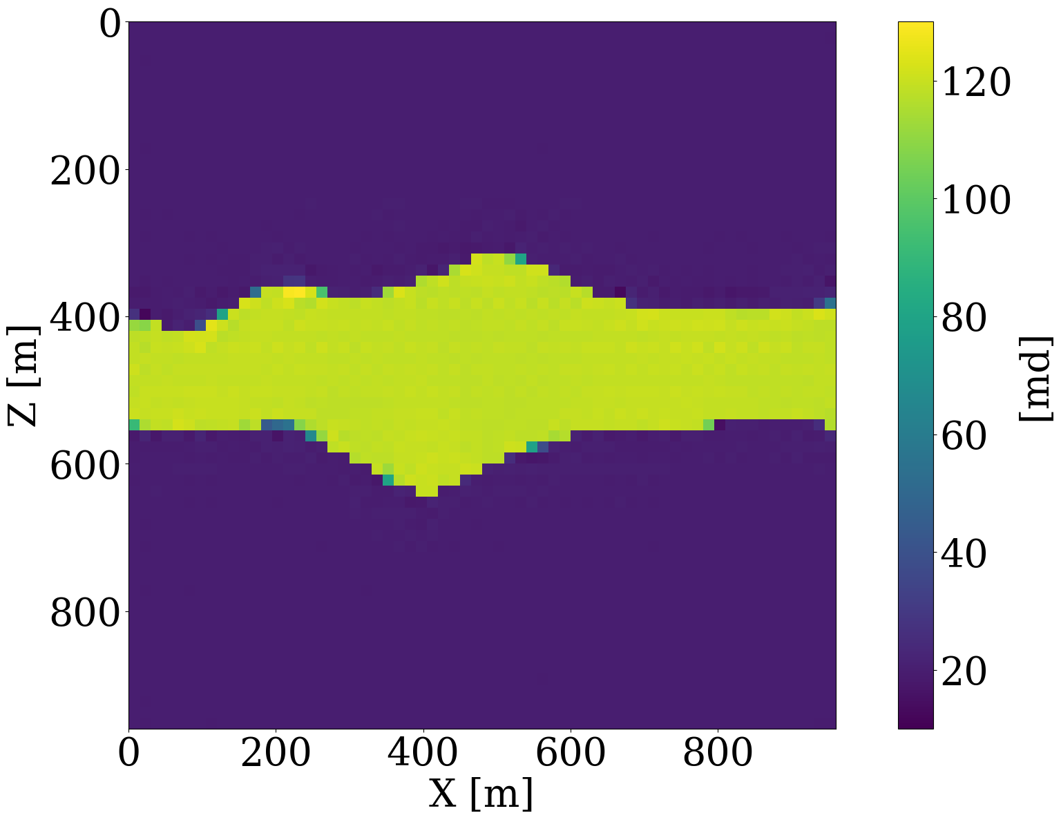
To better understand the behavior of a trained normalizing flow in conjunction with the \(\ell_2\)-norm constraint for in- and out-of-distribution examples, we include Figure 2 and Figure 3. In the latter Figure, nonlinear projections (via latent space shrinkage), \[ \widetilde{\mathbf{K}} = \mathcal{G}_{\mathbf{w}^\ast}\left(\alpha\mathbf{z}\right)\quad\text{where}\quad \mathbf{z}=\mathcal{G}_{\mathbf{w}^\ast}^{-1}(\mathbf{K}) \tag{6}\]
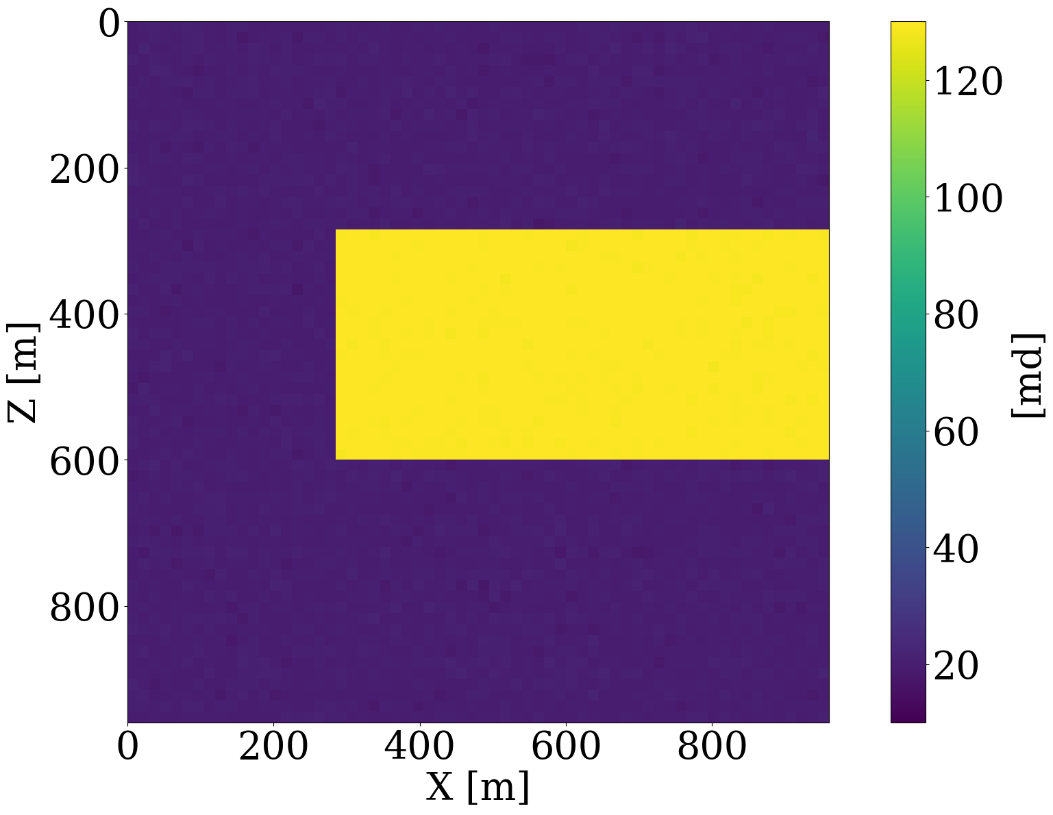
are plotted as a function of increasing \(\alpha\). We also plot in Figure 4 the NF’s relative nonlinear approximation error, \(\|\mathbf{\widetilde{K}}-\mathbf{K}\|_2/\|\mathbf{K}\|_2\), and the corresponding relative FNO prediction error,\(\|\mathcal{S}_{\boldsymbol\theta^\ast}(\widetilde{\mathbf{K}})-\mathcal{S}(\widetilde{\mathbf{K}})\|_2/\|\mathcal{S}(\widetilde{\mathbf{K}})\|_2\) as a function of increasing \(0\leq\alpha\leq 1\). From these plots, we can make the following observations. First, the latent representations (Figure 2 (c) and Figure 2 (d)) of the in- and out-of-distribution samples (Figure 2 (a) and Figure 2 (b) ) clearly show that NF applied to out-of-distribution samples produces a latent variable far from the standard normal distribution, while the latent variable corresponding to the in-distribution example is close to being white Gaussian noise. Quantitatively, the \(\ell_2\) norm of the latent variables are \(0.99\|\mathcal{N}(0,\mathbf{I})\|_2\) and \(3.11\|\mathcal{N}(0,\mathbf{I})\|_2\), respectively, where \(\|\mathcal{N}(0,\mathbf{I})\|_2\) corresponds to the \(\ell_2\)-norm of the standard normal distribution. Second, we observe from Figure 3 that for small \(\ell_2\)-norm balls (\(\alpha\ll 1\)) the projected solutions tend to be close to the most probable sample, which is a flat permeability channel in the middle. This is true for both the in- and out-of-distribution example. As \(\alpha\) increases, the in-distribution example is reconstructed accurately when the \(\ell_2\) norm of the scaled latent variable, \(\|\alpha\mathbf{z}\|_2\), is close to the \(\|\mathcal{N}(0,\mathbf{I})\|_2\). Clearly, this is not the case for the out-of-distribution example. When \(\|\alpha\mathbf{z}\|_2\approx\|\mathcal{N}(0,\mathbf{I})\|_2\), the reconstruction still looks like an in-distribution permeability sample and is not close to the out-of-distribution sample. However, if \(\alpha=1\), which makes \(\|\alpha\mathbf{z}\|_2\) well beyond the norm of the standard normal distribution, the out-of-distribution example is recovered accurately by virtue of the invertibility of NFs, irrespective on their input and what they have been trained on. Third, the relative FNO prediction error for the in-distribution example (Figure 4 (a)) remains flat while the error of the FNO surrogate increases as soon as \(\alpha\approx 0.25\). At that value for \(\alpha\), the projection, \(\widetilde{\mathbf{K}}\), is gradually transitioning from being in-distribution to out-of-distribution, which occurs at a non-linear approximation error of about 45%. As expected the plots in Figure 4 also show a monotonous decay of the nonlinear approximation error as a function of increasing \(\alpha\). To further analyze the effects of the nonlinear projections in Equation 6, we draw 50 random realizations from the standard normal distribution, scale each of them by \(0\leq\alpha\leq 2\), and calculate the FNO prediction errors on these samples. Figure 5 includes the results of this excercise where each column represents the FNO prediction error calculated for \(0\leq \alpha \leq 2\). From these experiments, we make the following two observations. First, when \(\alpha<0.8\), the FNO consistently makes accurate predictions for all projected samples. Second, as expected, the FNO starts to make less accurate predictions for \(\alpha>1\) with errors that increase as the size of the \(\ell_2\)-norm ball of the latent space expands, demarcating the transition from being in distribution to being out-of-distribution.


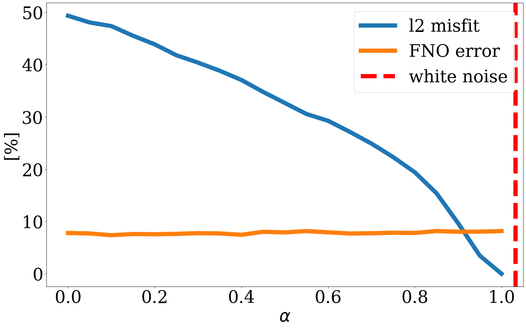
In summary, the experiments of Figure 2 to Figure 4 indicate that FNO errors remain small and relatively constant for the in-distribution example. Irrespective of the value of \(\alpha\), the generated samples remain in distribution while moving from the most likely—i.e., a flat high-permeability channel in the middle, to the in-distribution sample as \(\alpha\) increases. Conversely, the projection of the out-of-distribution example morphs from being in distribution to being out-of-distribution for \(\alpha \geq 0.25\). The FNO prediction errors also increase during this transition from an in-distribution sample to an out-of-distribution sample. Therefore, shrinkage in the latent space by multiplying with a small \(\alpha\) can serve as an effective projection that ensures relatively low FNO prediction errors. We will use this unique ability to control the distribution during inversion.
Inversion with progressively relaxed learned constraints
Our main objective is to perform inversions where the multiphase flow equations are replaced with pretrained FNO surrogates. To make sure the learned surrogates remain accurate, we propose working with a continuation scheme where the learned constraint in Equation 5 is steadily relaxed by increasing the size of the \(\ell_2\)-norm ball constraint. Compared to the more common penalty formulation, where regularization entails adding a Lagrange-multiplier weighted \(\ell_2\)-norm squared, constrained formulations offer guarantees that the model iterates for the latent variable, \(\mathbf{z}\), remain within the constraint set—i.e., within the \(\ell_2\)-norm ball of size \(\tau\). Using the argument of the previous section, this implies that permeability distributions generated by the trained NF remain in distribution as long as the size of the initial \(\ell_2\)-norm ball, \(\tau_{\mathrm{init}}\), is small enough (e.g., smaller than \(0.6\|\mathcal{N}(0,\mathbf{I})\|_2\), following the observations from Figure 5). Taking advantage of this trained NF in a homotopy, we propose the following algorithm:
Algorithm 1: Inversion with relaxed learned constraints
1. Input: initial model parameter \(\mathbf{K}_0\in \mathbb{R}^N\), observed data \(\mathbf{d}\), noise level \(\sigma\)
2. Input: trained FNO \(\mathcal{S}_{\boldsymbol{\theta}^\ast}\), trained NF \(\mathcal{G}_{\mathbf{w}^\ast}\)
3. Input: number of inner-loop iterations \(maxiter\)
4. Input: initial \(\ell_2\) ball size \(\tau_{\mathrm{init}}\), multiplier \(\beta>1\), final \(\ell_2\) ball size \(\tau_{\mathrm{final}}\)
5. \(\mathbf{z} = \mathcal{G}_{\mathbf{w}^\ast}^{-1}(\mathbf{K}_0)\)
6. \(\tau = \tau_{\mathrm{init}}\)
7. while \(\|\mathbf{d} - \mathcal{H}\circ\mathcal{S}_{\boldsymbol\theta^\ast}\circ\mathcal{G}_{\mathbf{w}^\ast}(\mathbf{z})\|_2 > \sigma\|\mathcal{N}(0,\mathbf{I})\|_2\) and \(\tau\leq\tau_{\mathrm{final}}\)
8. for \(iter = 1:maxiter\)
9. \(\displaystyle\mathbf{g}=\nabla_{\mathbf{z}}\|\mathbf{d} - \mathcal{H}\circ\mathcal{S}_{\boldsymbol\theta^\ast}\circ\mathcal{G}_{\mathbf{w}^\ast}(\mathbf{z})\|_2^2\)
10. \(\mathbf{z} = \mathcal{P}_{\tau}(\mathbf{z} - \gamma\mathbf{g})\)
11. end
12. \(\tau = \beta\tau\)
13. end
14. Output: inverted model parameter \(\mathbf{K}=\mathcal{G}_{\mathbf{w}^\ast}(\mathbf{z})\)
Given observed data, \(\mathbf{d}\), trained networks, \(\mathcal{S}_{\boldsymbol{\theta}^\ast}\) and \(\mathcal{G}_{\mathbf{w}^\ast}\), the initial guess for the permeability distribution, \(\mathbf{K} _0\), the initial size of the \(\ell_2\)-norm ball, \(\tau_{\mathrm{init}}\), and the final size of the \(\ell_2\)-norm ball, \(\tau_{\mathrm{final}}\), Algorithm 1 proceeds by solving a series of constrained optimization problems where the size of the constraint set is increased by a factor of \(\beta\) after each iteration (cf. line 12 in Algorithm 1). The constrained optimization subproblems themselves (cf. line 8 to 11 of Algorithm 1) are solved with projected gradient descent (Beck 2014). Each iteration of the projected gradient descent method first calculates the gradient (cf. line 9 of Algorithm 1), followed by the much cheaper projection of the updated latent variable back onto the \(\ell_2\)-norm ball of size \(\tau\) via the projection operator \(\mathcal{P}_{\tau}\) (cf. line 10 in Algorithm 1). This projection is a trivial scaling operation if the updated latent variable \(\ell_2\)-norm exceeds the constraint — i.e., \[ \mathcal{P}_{\tau}(\mathbf{z}) = \begin{cases} \mathbf{z} & \text{if } \|\mathbf{z}\|_2 \leq \tau \\ \tau\mathbf{z}/\|\mathbf{z}\|_2 & \text{if } \|\mathbf{z}\|_2 > \tau \end{cases} \tag{7}\]
A line search determines the steplength \(\gamma\) (Stanimirović and Miladinović 2010) for each iteration shown in line 8 to 11. As is common in continuation methods, the relaxed gradient-descent iterations are warm-started with the optimization result from the previous iteration, which at the first iteration is initialized by the latent representation of the initial permeability model, \(\mathbf{K}_0\) (cf. line 5 in Algorithm 1). Practically, each subproblem does not need to be fully solved, but only need a few iterations instead. The number of iterations to solve each subproblem is denoted by \(maxiter\) in line 8 of Algorithm 1. This continuation strategy serves two purposes. First, for small \(\tau\)’s it makes sure the model iterates remain in distribution, so accuracy of the learned surrogate is preserved. Second, by relaxing the constraint slowly, the data residual is gradually allowed to decrease, bringing in more and more features derived from the data. By slowly relaxing the constraint, we find a careful balance between these two purposes as long as progress is made towards the solution when solving the subproblem (cf. line 8 to 11 in Algorithm 1). One notable distinction of the surrogate-assisted inversion, compared to the conventional inversion with relaxed constraints (Esser et al. 2018), is that the size of the \(\ell_2\)-norm projection ball cannot increase far beyond the \(\ell_2\)-norm of the standard Gaussian white noise on which the NFs are trained. Otherwise, there is no guarantee the learned surrogate is accurate because the NF may generate samples that are out-of-distribution (cf. Figure 5). This is explicitly incorporated into the stopping criteria, \(\tau\leq\tau_{\mathrm{final}}\), in line 7 of Algorithm 1.
Numerical Experiments
To showcase the advocasy of the proposed optimization method with relaxed learned constraints, a series of carefully chosen experiments of increasing complexity are conducted. These experiments are designed to be relevant to GCS, which in its ultimate form involves coupling of multiphase flow with the wave equation to perform end-to-end inversion for the permeability given multimodal data. To convince ourselves of the validity of our approach, at all times comparisons will be made between inversion results involving numerical solves of the multiphase equations and inversions yielded by approximations with our learned surrogate.
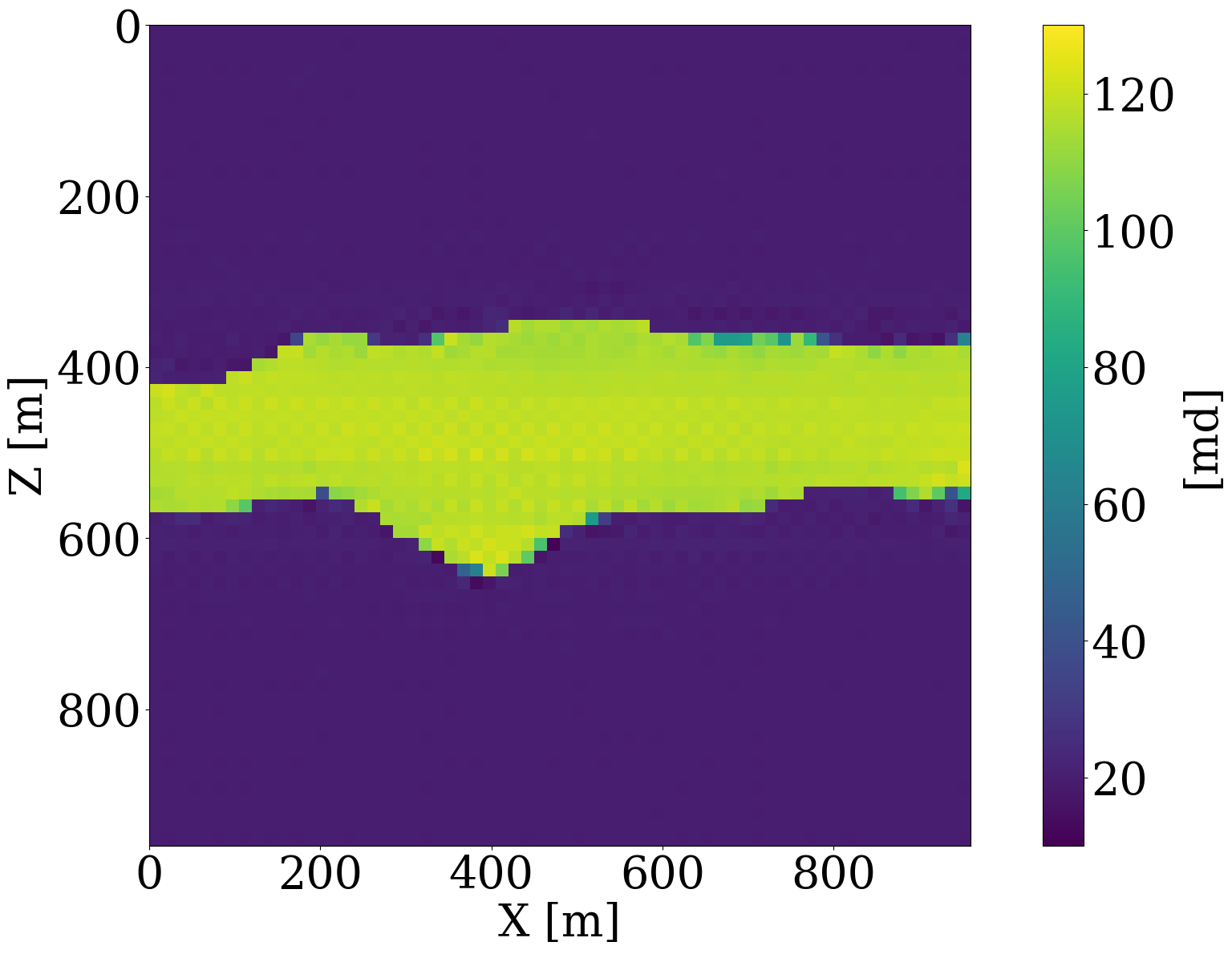
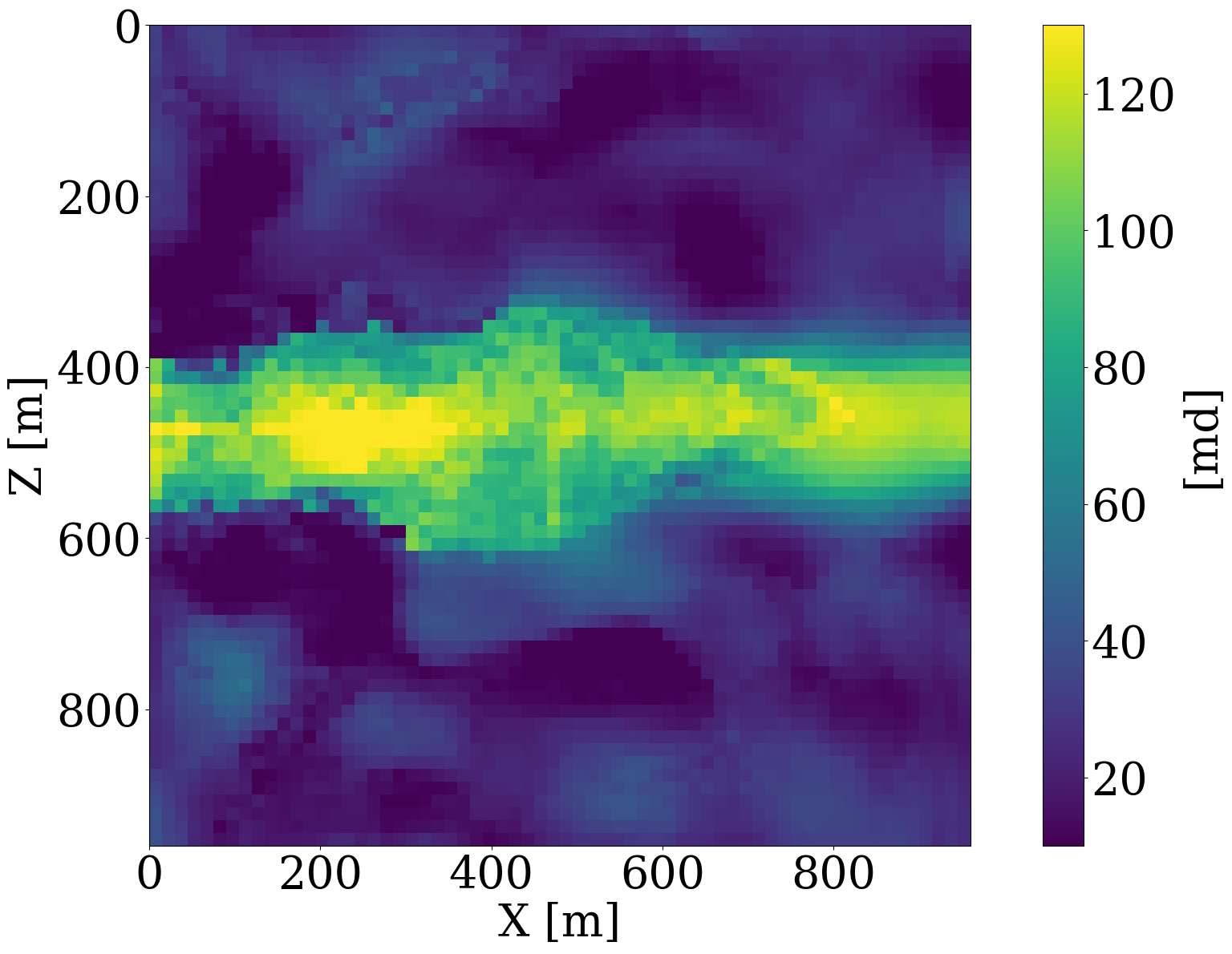
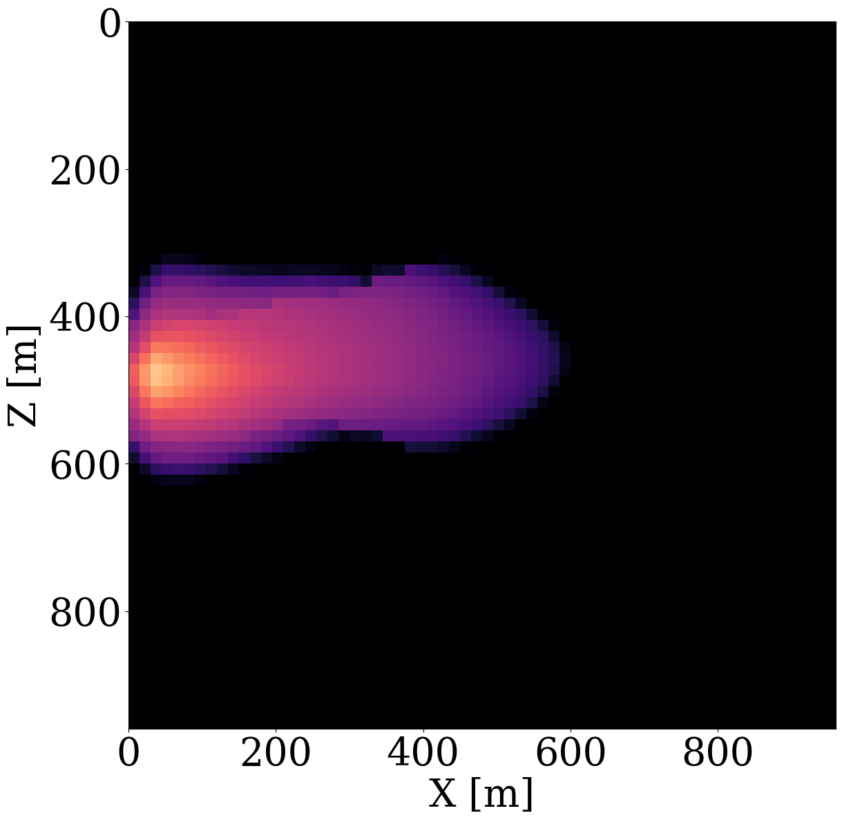
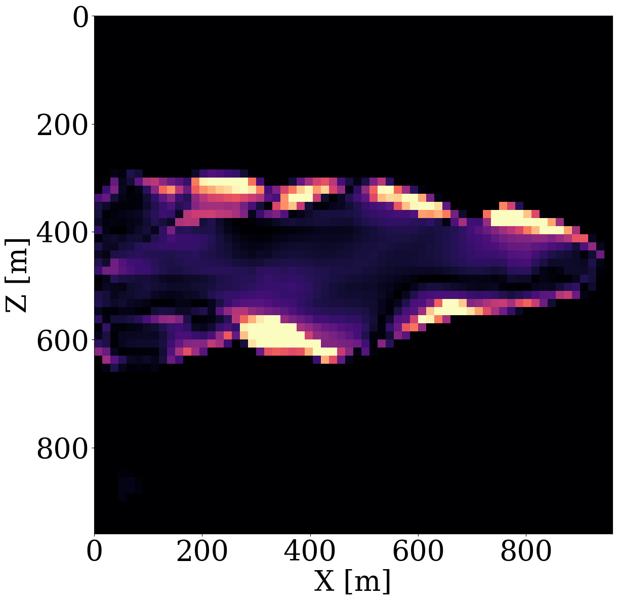
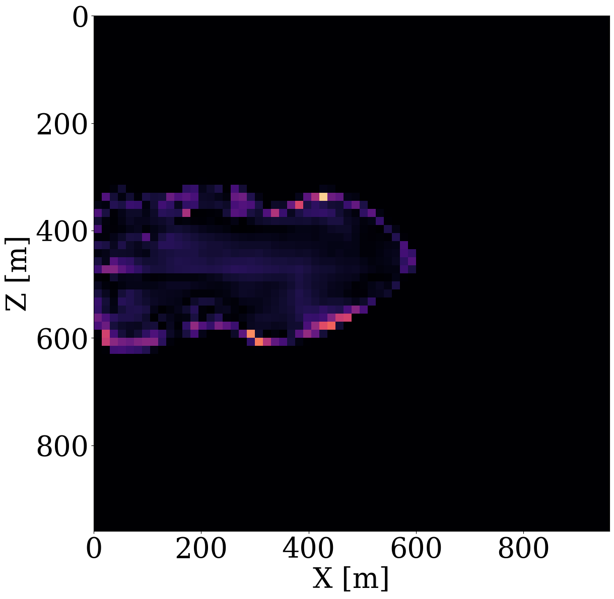
For all numerical experiments, the “ground-truth” permeability model will be selected from the unseen test set and is shown in Figure 6 (a). The inversions will be initiated with the smooth permeability model depicted in Figure 6 (b). This initial model, \(\mathbf{K}_0\), represents the arithmetic mean of all permeability samples in the training dataset. To ensure that the model iterates remain in distribution, we set the starting \(\ell_2\)-norm ball size to \(\tau_{\mathrm{init}}=0.6 \|\mathcal{N}(0,\mathbf{I})\|_2\)—i.e., \(0.6\times\) the \(\ell_2\)-norm of standard white Gauss noise realizations for the discrete permeability model of 64 by 64 gridpoints. To gradually relax the learned constraint, the multiplier of the projection ball size is taken to be \(\beta=1.2\), and we set the ultimate projection ball size \(\tau_{\mathrm{final}}\) in Algorithm 1 to be \(1.2\) times the norm of standard white noise. To limit computational costs of solving the subproblems, we allow each constrained subproblem (cf. line 8 to 11 in Algorithm 1) to perform 8 iterations of projected gradient descent to solve for the latent variable. From practical experience, we found that the proposed inversions are not very sensitive to the choice of these hyperparameters.
To simulate the evolution of injected CO2 plumes, we make use of the open-source software package Jutul.jl (Møyner et al. 2023; Møyner, Bruer, and Yin 2023; Yin, Bruer, and Louboutin 2023), which for each permeability model, \(\mathbf{K}^{(j)}\), solves the immiscible and compressible two-phase flow equations for the CO2 and brine saturation. As shown in Figure 6 (a), an injection well is set up on the left-hand side of the model, which injects supercritical CO2 with density 700 \(\mathrm{kg}/\mathrm{m}^3\) at a constant rate of 0.005 \(\mathrm{m}^3/\mathrm{s}\). To relieve pressure, a production well is included on the right-hand side of the model, which produces brine with density 1000 \(\mathrm{kg}/\mathrm{m}^3\) with a constant rate of also 0.005 \(\mathrm{m}^3/\mathrm{s}\). This finally results in approximately a \(6\%\) storage capacity after 800 days of CO2 injection. From these simulations, we collect eight snapshots for the CO2 concentration, \(\mathbf{c}=[\mathbf{c}_1, \mathbf{c}_2, \cdots,\mathbf{c}_{n_t}]\) with \(n_t=8\) the number of snapshots that cover a total time period of 800 days. The last five snapshots of these simulations are included in the top row of Figure 6 (a). Due to buoyancy effects and well control, the CO2 plume gradually moves from the left to the right and upwards.


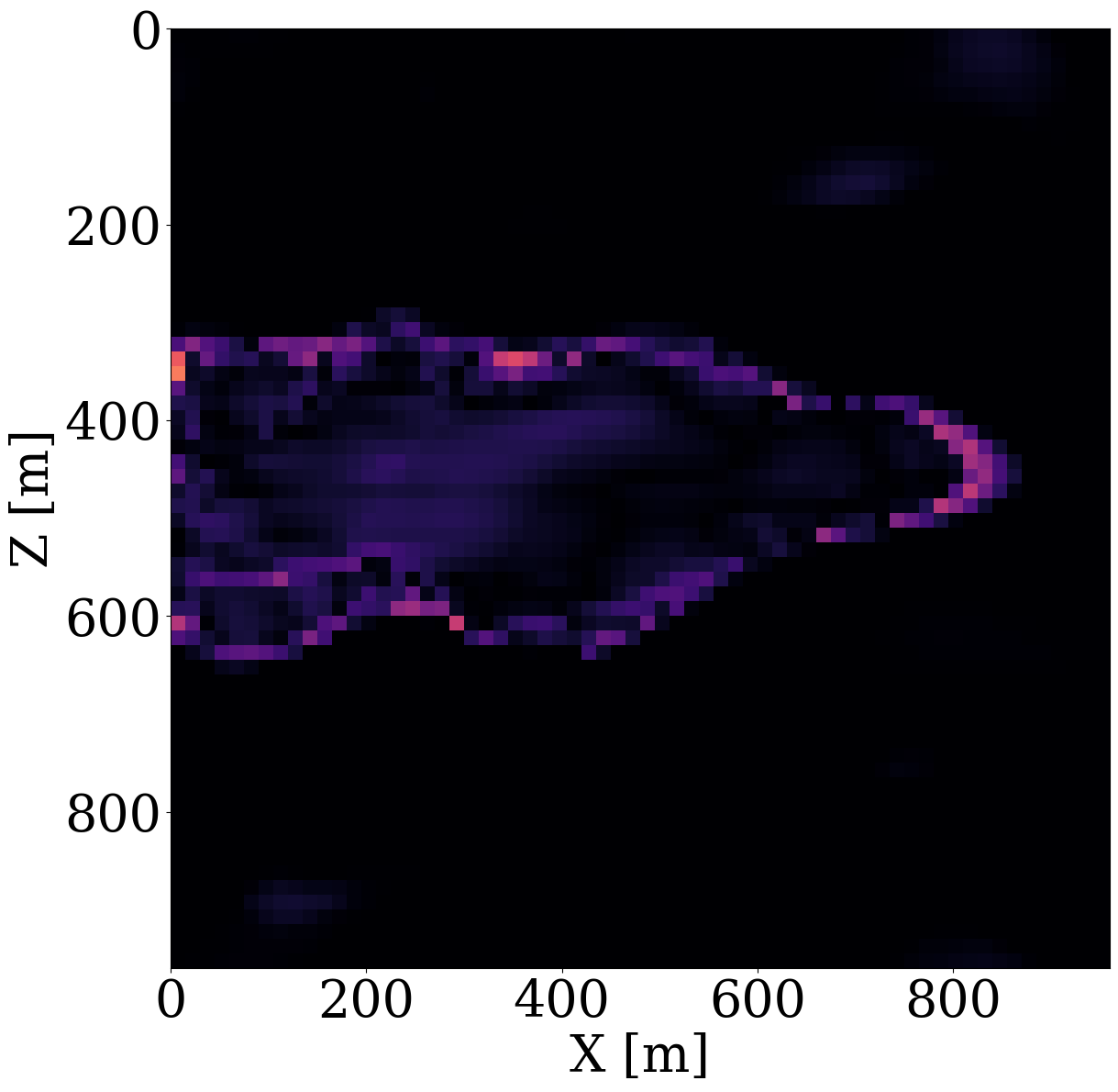
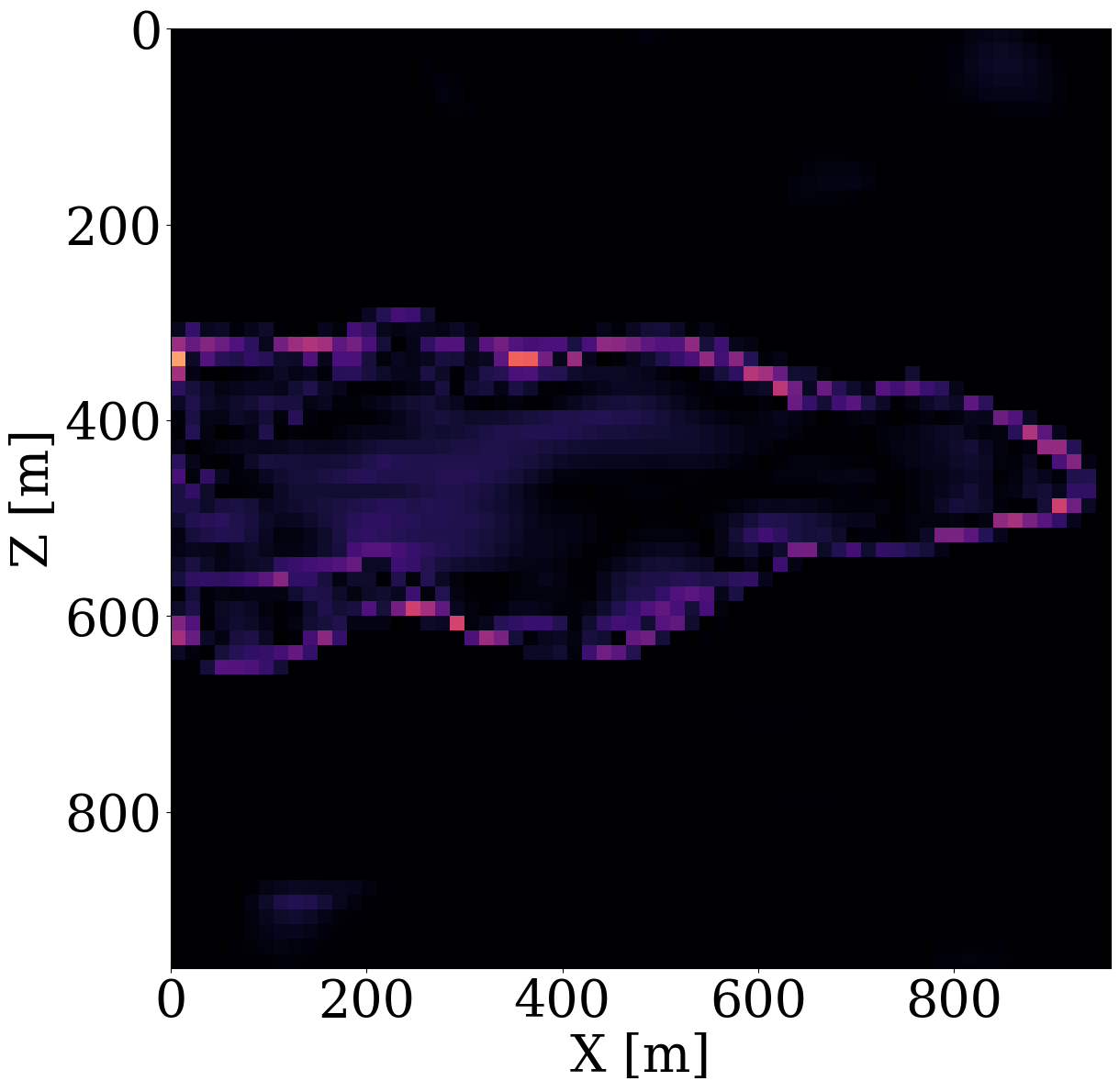
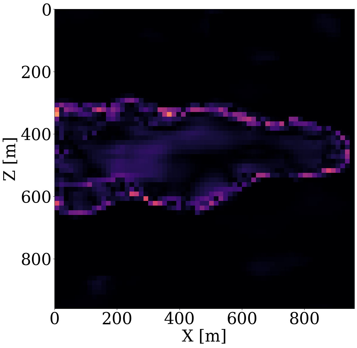
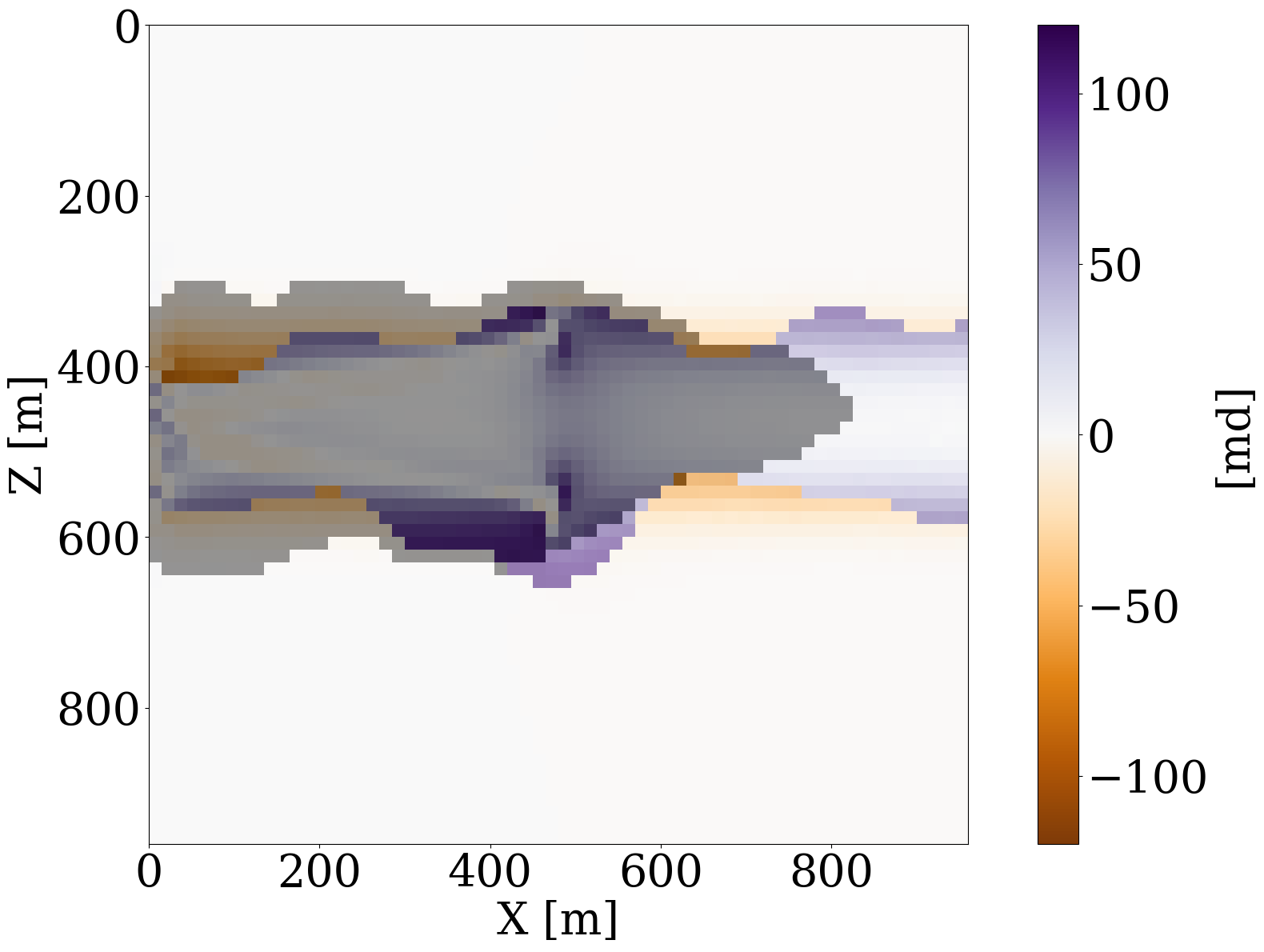
Given these simulated CO2 concentrations, the optimized weights, \(\mathbf{w}^\ast\), for the FNO surrogate are calculated by minimizing Equation 2 for \(N=1900\) training pairs, \(\{\mathbf{K}^{(j)},\, \mathbf{c}^{(j)}\}_{j=1}^N\). Another 100 training pairs are used for validation. After training with 350 epochs, an average of 7% prediction error is achieved for permeability samples from the unseen test set. As observed from Figure 7, the approximation errors of the FNO are mostly concentrated at the leading edge of the CO2 plumes. The same permeability models are used to train the NF by minimizing Equation 4 for 245 epochs using the open-source software package InvertibleNetworks.jl (P. Witte et al. 2023). We use the HINT network structure (Kruse et al. 2021) for the NF. Three generative samples are shown in the second row of Figure 1. From these examples, we can see that the trained NF is capable of generating random permeability models that resemble the ones in the training samples closely, despite minor noisy artifacts.
Unconstrained/constrained permeability inversion from CO2 saturation data
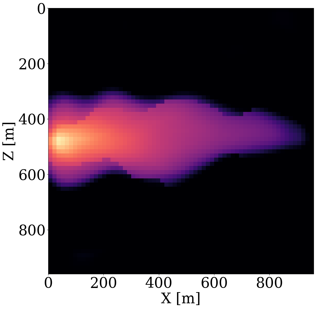
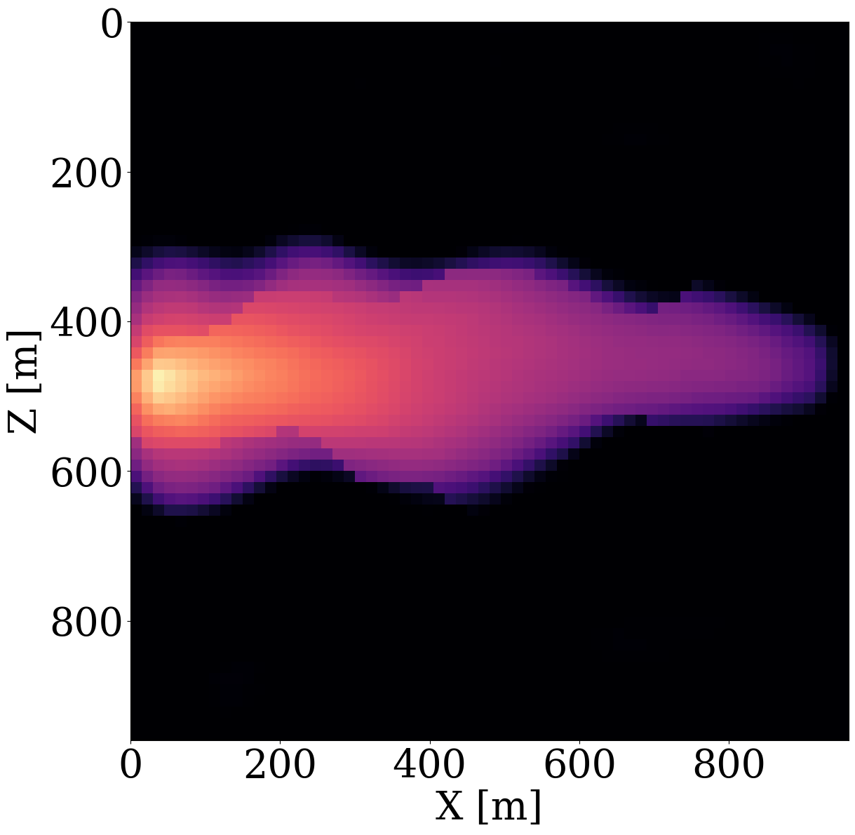
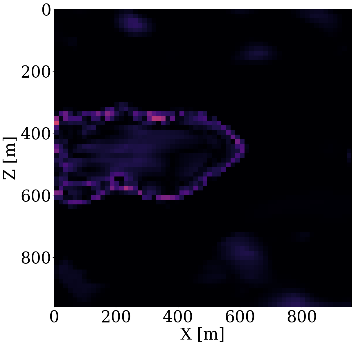
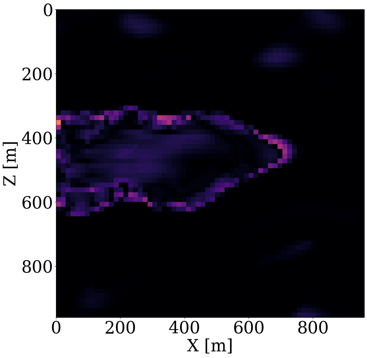
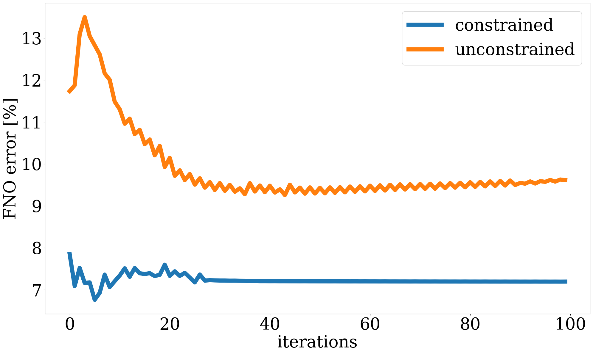
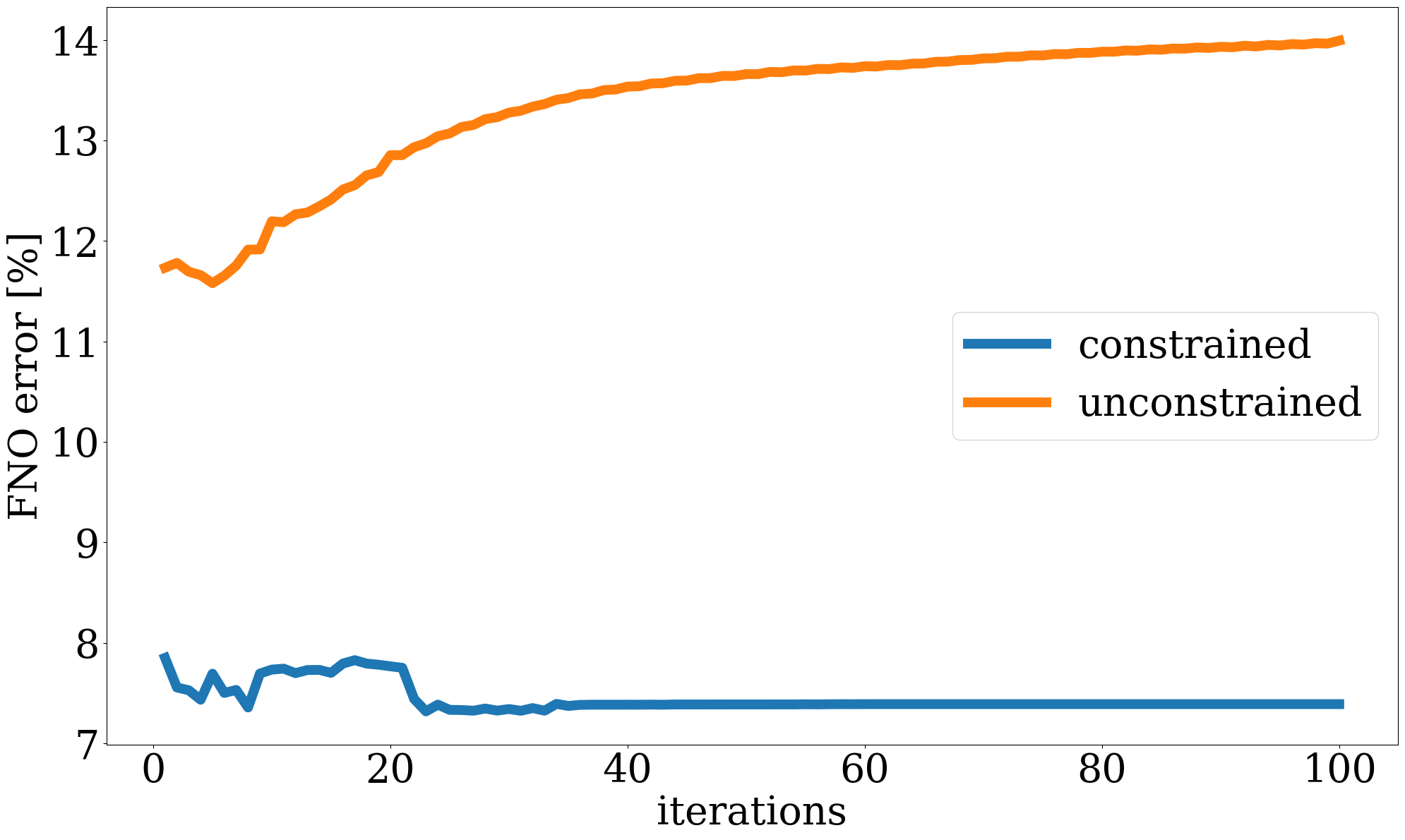
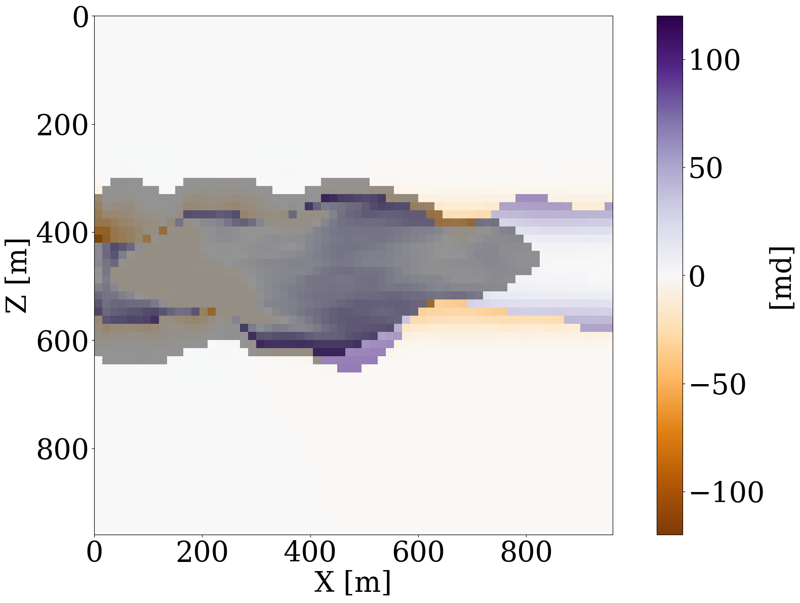
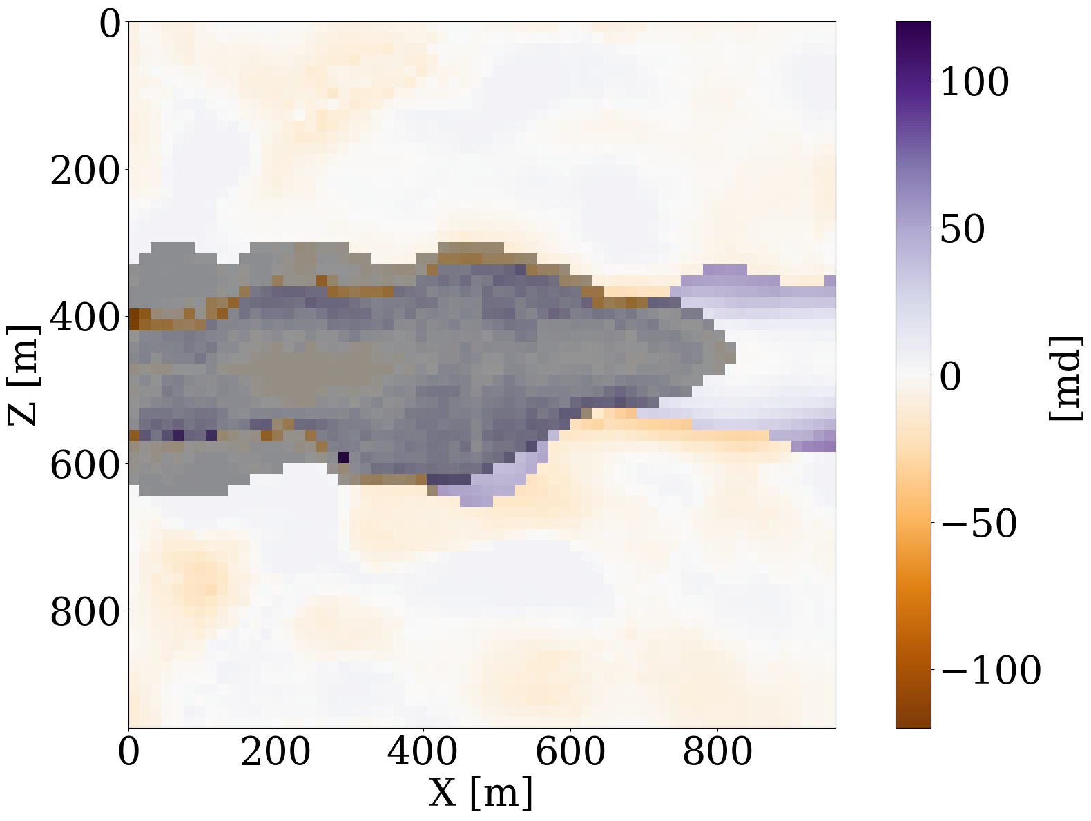
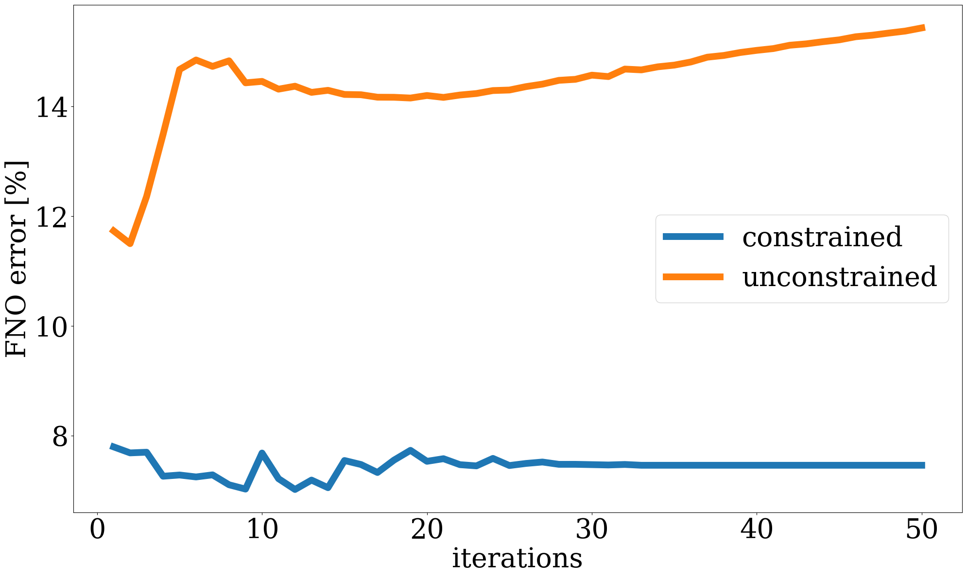
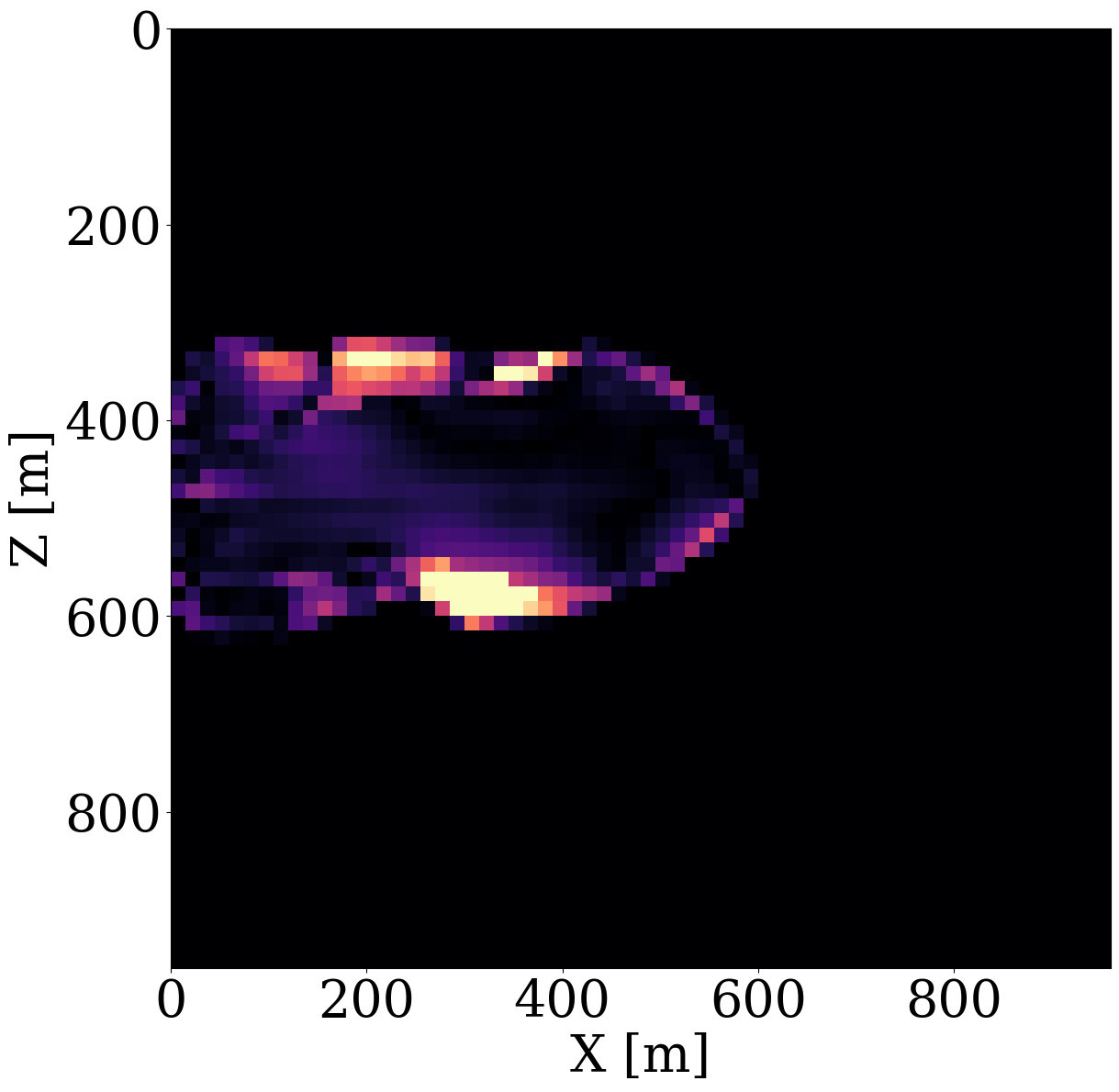
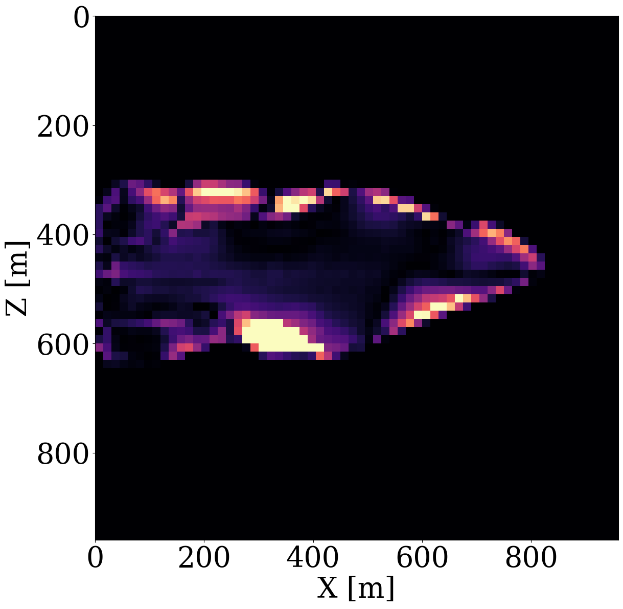
To demonstrate that permeability inversion with surrogates is indeed feasible, we first consider the idealized, impossible in practice, situation where we assume to have access to the time-lapse CO2 concentration, \(\mathbf{c}=[\mathbf{c}_1, \mathbf{c}_2, \cdots,\mathbf{c}_{n_t}]\), everywhere, and for all \(n_t=8\) timesteps. In that case, the measurement operator, \(\mathcal{H}\) in Equation 1, corresponds to the identity matrix. Given CO2 concentrations simulated from the “ground-truth” permeability distribution plotted in Figure 6 (a), we invert for the permeability by minimizing the unconstrained formulation (cf. Equation 3) for the correct, yielded by the PDE, and approximate fluid-flow physics, yielded by the trained FNO. The results of these inversions after 100 iterations of gradient descent with back-tracking linesearch (Stanimirović and Miladinović 2010) are plotted in Figure 8 (a) and Figure 8 (b). From these plots, we observe that the inversion results using PDE solvers delineates most of the upper boundary of the channel accurately. Because there is a null space in the fluid-flow modeling—i.e., this null space mostly corresponds to regions of the permeability model that are barely touched by the CO2 plume (e.g. bottom and right-hand side of the channel) — artifacts are present in the high-permeability channel itself. As expected, the reconstruction of the permeability is also not perfect at the bottom and at the far right of the model. The inversion result with the FNO surrogate is similar but introduces unrealistic artifacts in the high-permeability channel and also outside the channel. These more severe artifacts can be explained by the behavior of the FNO approximation error plotted as the orange curve in Figure 8 (e). The error value increases rapidly to 13%, and finally saturates at 10%. This behavior of the error is a manifestation of out-of-distribution model iterates that explain the erroneous behavior of the surrogate and its gradient with respect to the permeability.
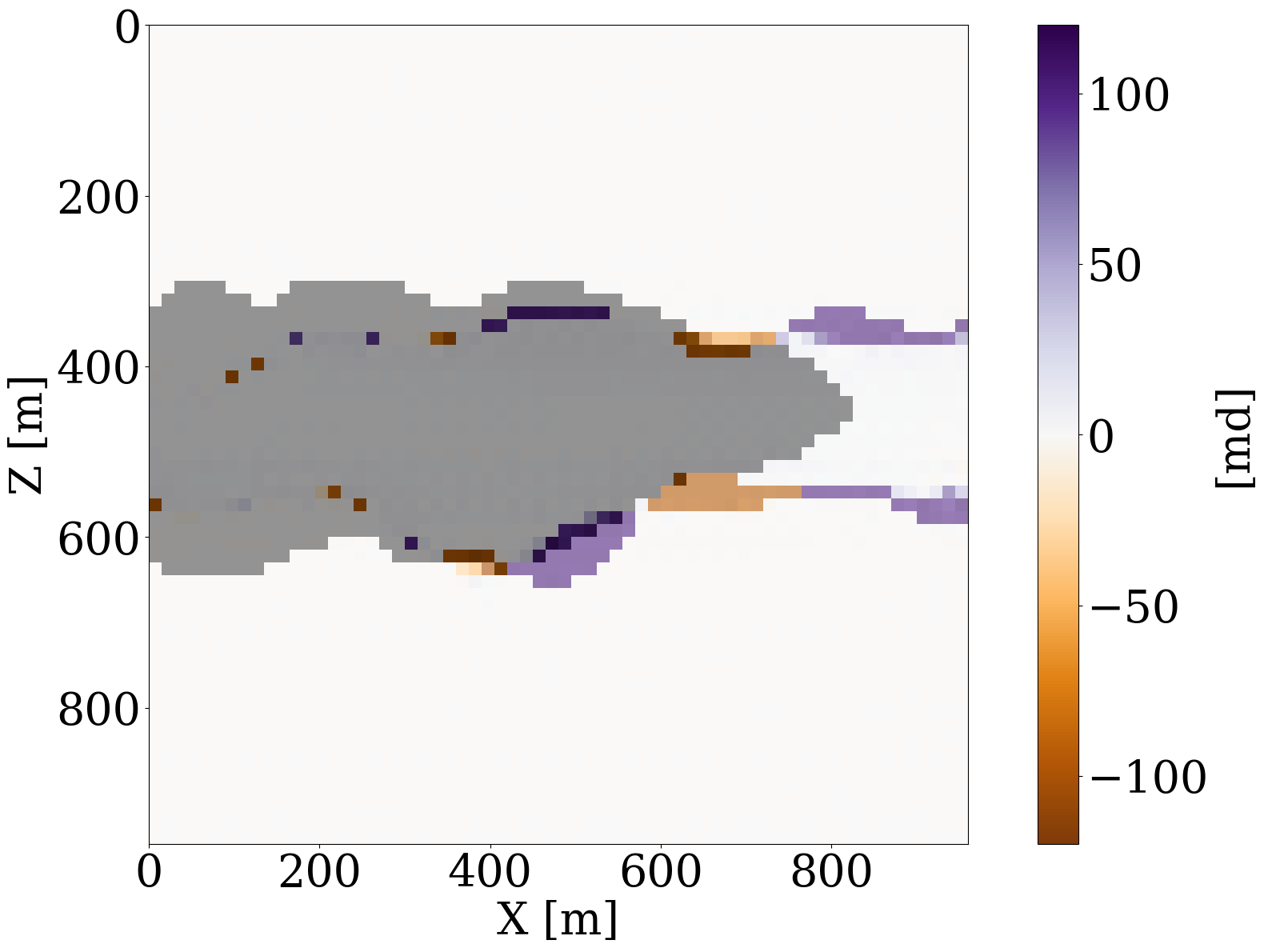
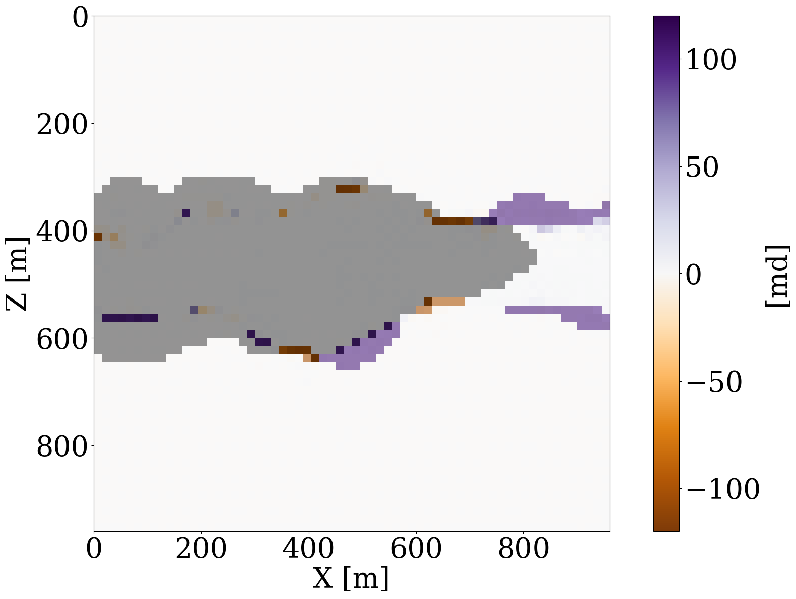
Inversions yielded by the relaxed constrained formulation with the trained NF (see Algorithm 1), on the other hand, show virtually artifact free inversion results (see Figure 8 (c) and Figure 8 (d)) that compare favorably with the “ground-truth” permeability plotted in Figure 6. While adding the NF as a constraint obviously adds information, explaining the improved inversion for the accurate physics (Figure 8 (c)), it also renders the approximate surrogates more accurate, as can be observed from the blue curve in Figure 8 (e), where the FNO approximation error is controlled thanks to adding the constraint to the inversion. This behavior underlines the importance of ensuring model iterates to remain within distribution. It also demonstrates the benefits of a solution strategy where we start with a small \(\tau\), followed by relaxing the constraint slowly by increasing the size of the constraint set gradually.


Unconstrained/constrained permeability inversion from well observations
While the example of the previous section established feasibility of constrained permeability inversion, it relied on having access to the CO2 saturation everywhere, which is unrealistic in practice. To address this issue, we first consider permeability inversion from CO2 saturations, collected at three equally spaced monitoring well locations, for only the first 6 timesteps over the period of 600 days (Mosser, Dubrule, and Blunt 2019). In this more realistic setting, the measurement operator, \(\mathcal{H}\) in Equation 1, corresponds to a restriction operator that extracts simulated CO2 saturations at each well location in first six snapshots. The objective function reads
\[ \underset{\mathbf{z}}{\operatorname{minimize}} \quad \|\mathbf{d}_{\mathrm{w}}-\mathbf{M}\circ\mathcal{S}_{\boldsymbol\theta^\ast}\circ\mathcal{G}_{\mathbf{w}^\ast}(\mathbf{z})\|_2^2\quad\text{subject to}\quad\|\mathbf{z}\|_2\leq \tau, \tag{8}\]
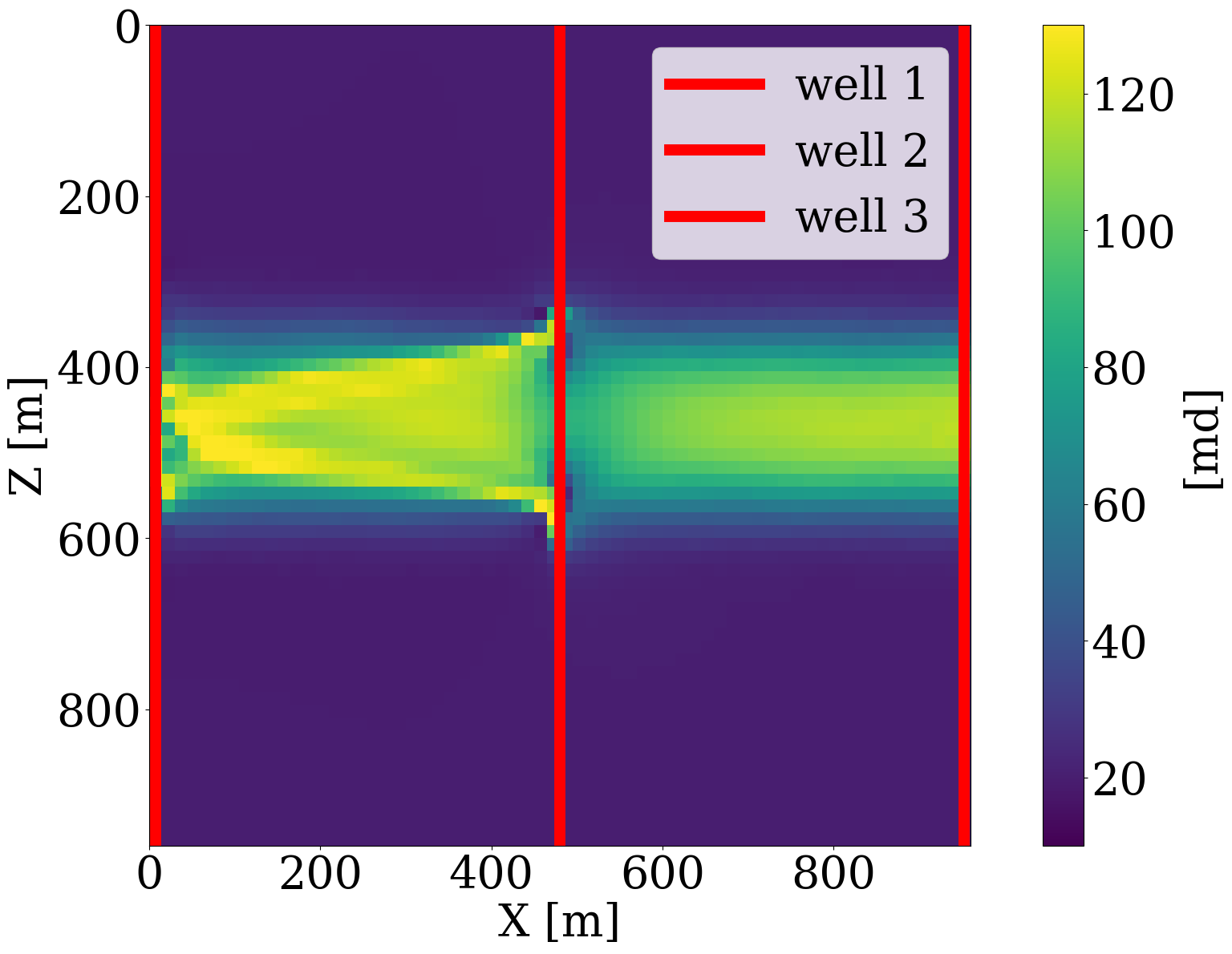
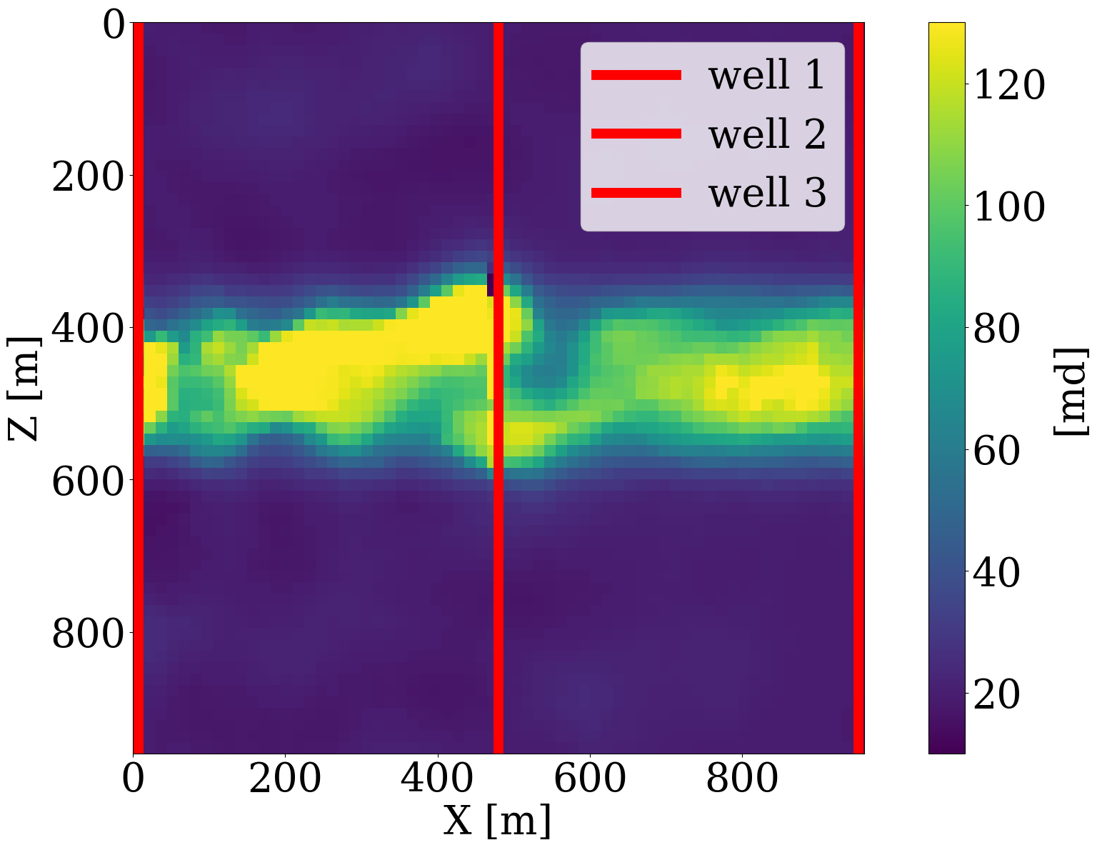
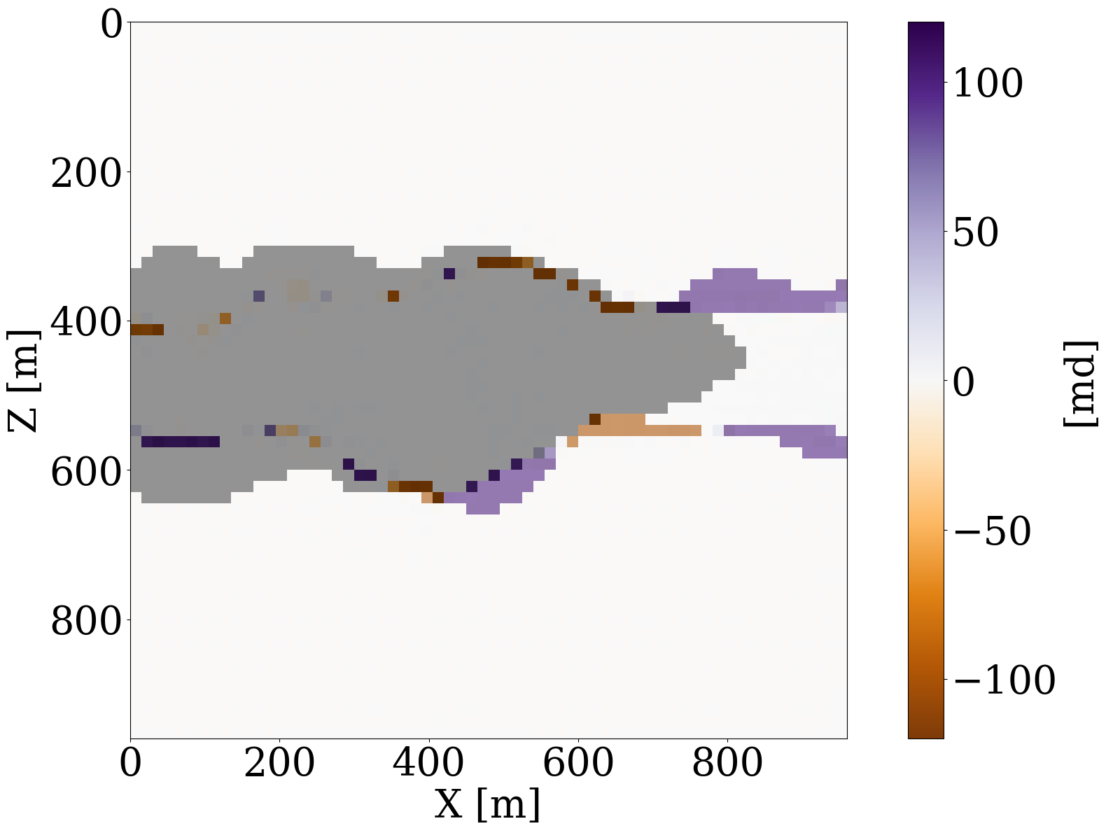
where \(\mathbf{d}_{\mathrm{w}}\) represents the well measurements collected at three well locations through the linear restriction operator \(\mathbf{M}\). The goal is to invert for the permeability by minimizing the misfit of the well measurements of the CO2 saturation without and with constraints on the \(\ell_2\)-norm ball in the latent space. The results of these numerical experiments are included in the first row of Figure 9, where the differences with respect to the ground truth permeability shown in Figure 6 (a) are plotted in the second row. Because the part of the permeability that is not touched by the CO2 plume lives in the null space, we highlight the CO2 plume in the difference plots by dark color and focus on analyzing errors within the plume region. As expected, the unconstrained inversions based on PDE solves (Figure 9 (a)) and surrogate approximations (Figure 9 (b)) are both poorly resolved because of the limited spatial information on the saturation. Contrasting these unconstrained inversions with results for the constrained inversions for the PDE (Figure 9 (c)) and surrogate (Figure 9 (d)) again shows the importance of adding constraints to the inversion. Figure 9 (i) clearly demonstrates that the FNO prediction errors remain relatively constant during constrained inversion while the error continues to grow during the unconstrained iterations eventually exceeding 14%. Both constrained results improve significantly, even though they converge to different solutions in the end. This is because history matching is typically an ill-posed problem with many distinctive solutions (Canchumuni, Emerick, and Pacheco 2019). This observation further motivates us to consider the experiment below, where time-lapse seismic data are jointly inverted for the subsurface permeability.


Multiphysics end-to-end inversion
Next, we consider the alternative setting for seismic monitoring of geological carbon storage, where the dynamics of the CO2 plumes are indirectly observed from time-lapse seismic data. In this case, the measurement operator, \(\mathcal{H}\), involves the composition of the rock physics modeling operator, \(\mathcal{R}\), which converts CO2 saturations to decreases in the compressional wavespeeds for rocks within the reservoir (Avseth, Mukerji, and Mavko 2010), and the seismic modeling operator, \(\mathcal{F}\), which generates time-lapse seismic data recorded at the receiver locations and based on acoustic wave equation modeling (Sheriff and Geldart 1995). The multiphysics end-to-end inversion process estimates permeability from time-lapse seismic data via inversion of these nested physics operators for the flow, rock physics, and waves (D. Li et al. 2020). Following earlier work by Yin et al. (2022) and Louboutin, Yin, et al. (2023), the fluid-flow PDE modeling is replaced by the trained FNO (cf. Equation 5), resulting in the following optimization problem:
\[ \underset{\mathbf{z}}{\operatorname{minimize}} \quad \|\mathbf{d}_{\mathrm{s}} - \mathcal{F}\circ\mathcal{R}\circ\mathcal{S}_{\boldsymbol\theta^\ast}\circ\mathcal{G}_{\mathbf{w}^\ast}(\mathbf{z})\|_2^2 \quad\text{subject to}\quad\|\mathbf{z}\|_2\leq \tau, \tag{9}\]
where \(\mathbf{d}_{\mathrm{s}}\) represents the observed time-lapse seismic data. While this end-to-end inversion problem benefits from having remote access to changes in the compressional wavespeed, it may now suffer from null spaces associated with the flow, \(\mathcal{S}_{\boldsymbol\theta^\ast}\), and the wave/rock physics, \(\mathcal{F}\circ\mathcal{R}\). For instance, the latter suffers from bandwidth limitation of the source function and from limited aperture. Because important components are missing in the observed data, inversion based on the data objective alone in Equation 9 are likely to suffer from artifacts that can easily drive the intermediate permeability model iterates out-of-distribution.
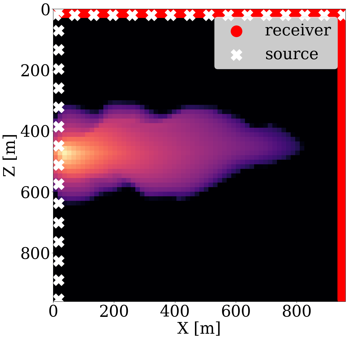
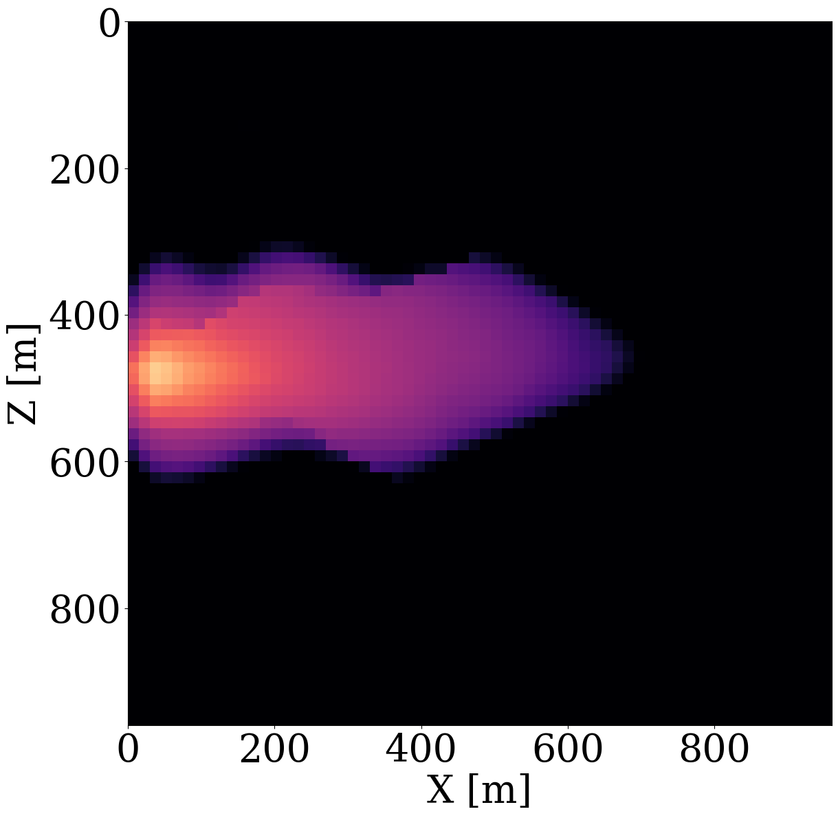
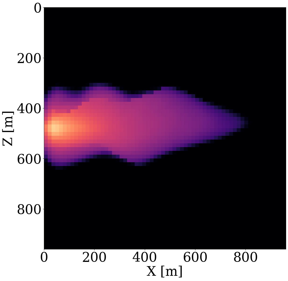
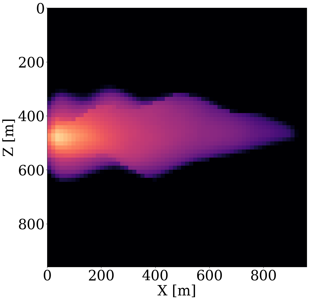
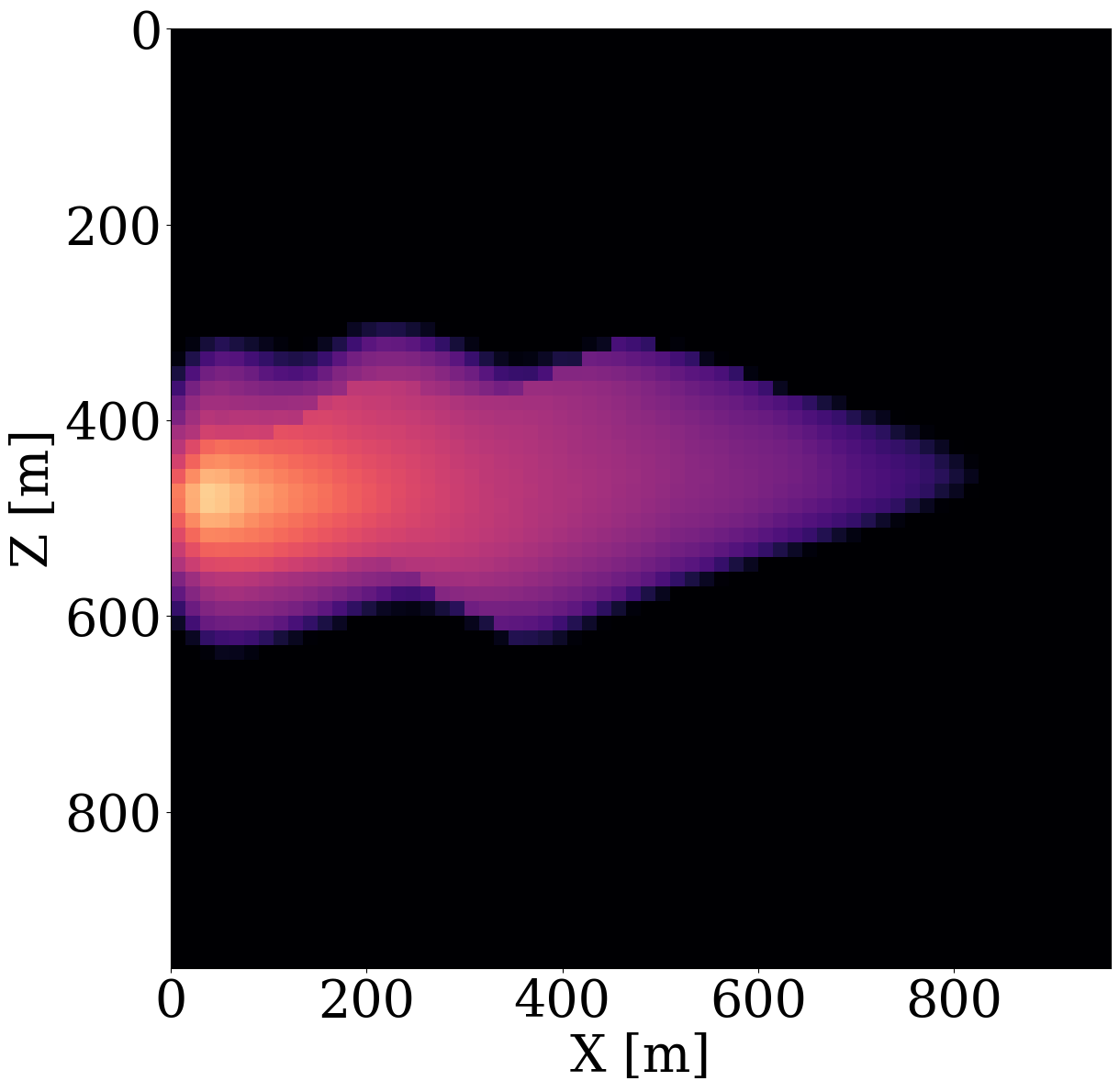
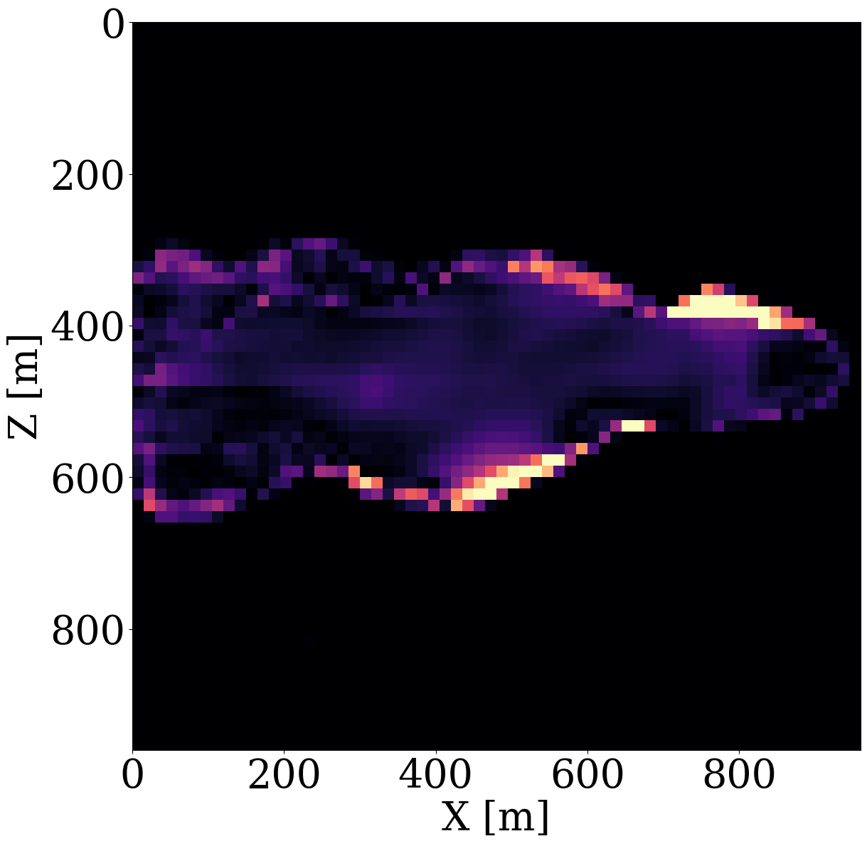
To demonstrate capabilities of the proposed relaxed inversion procedure with surrogates for the fluid flow, we assume the baseline to be known—i.e, we assume the brine-filled reservoir with \(25\%\) porosity to be acoustically homogeneous prior to CO2 injection with a compressional wavespeed of \(3500 \mathrm{m/s}\). We use the patchy saturation model (Avseth, Mukerji, and Mavko 2010) to convert the time-dependent CO2 saturation resulting in \(<300\mathrm{m/s}\) decreases in the wavespeed within the CO2 plumes. We collect six seismic surveys at the first six snapshots for the CO2 saturation from day 100 to day 600, which are the same snapshots as the ones used in the previous experiment. For each time-lapse seismic survey, 16 active-seismic sources are located within a well on the left-hand side of the model. We also position 16 sources on the top of the model. Each active source uses a Ricker wavelet with a central frequency of \(50\mathrm{Hz}\). The transmitted and reflected wavefields are collected by 480 receivers on the top and 480 receivers on the right-hand side of the model. The seismic acquisition is shown in Figure 10, where the plume at the last seismic vintage (at day 600) is plotted in the middle.
To avoid numerical dispersion, the velocity model is upsampled by a factor of two in both the horizontal and vertical directions, which results in a \(7.5\mathrm{m}\) grid spacing. For the simulations, use is made of the open-source software package JUDI.jl (Philipp A. Witte et al. 2019; Louboutin, Witte, et al. 2023) to generate the time-lapse seismic data at the first six snapshots. The fact that this software is based on Devito’s wave propagators (Louboutin et al. 2019; Luporini et al. 2020) allows us to do this quickly. For realism, we add 10 dB Gaussian noise to the time-lapse seismic data. Given these six time-lapse vintages, our goal is to invert for the permeability in the reservoir by minimizing the time-lapse seismic data misfit through the nested physics operators shown in Equation 9.


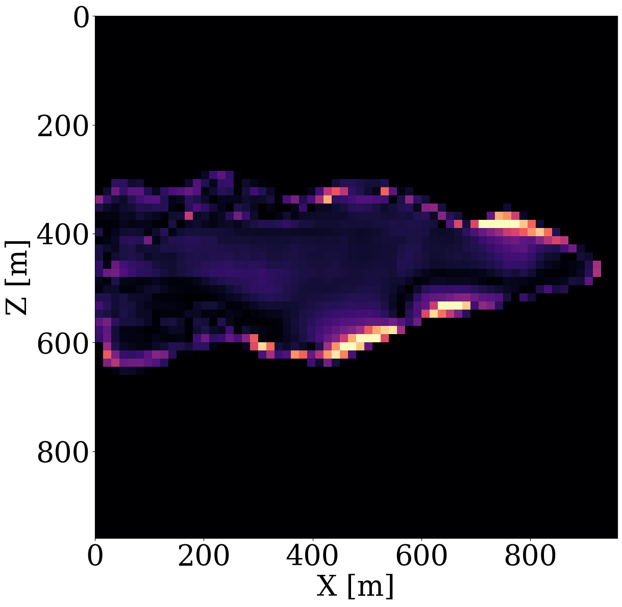
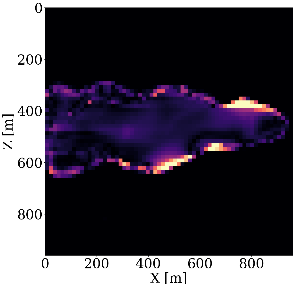
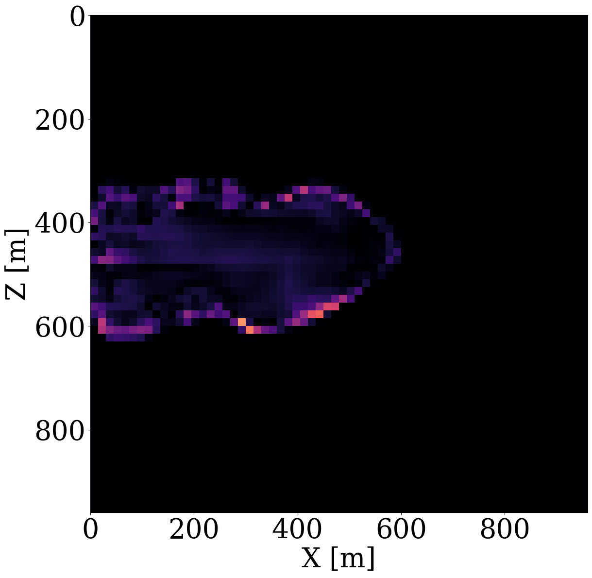
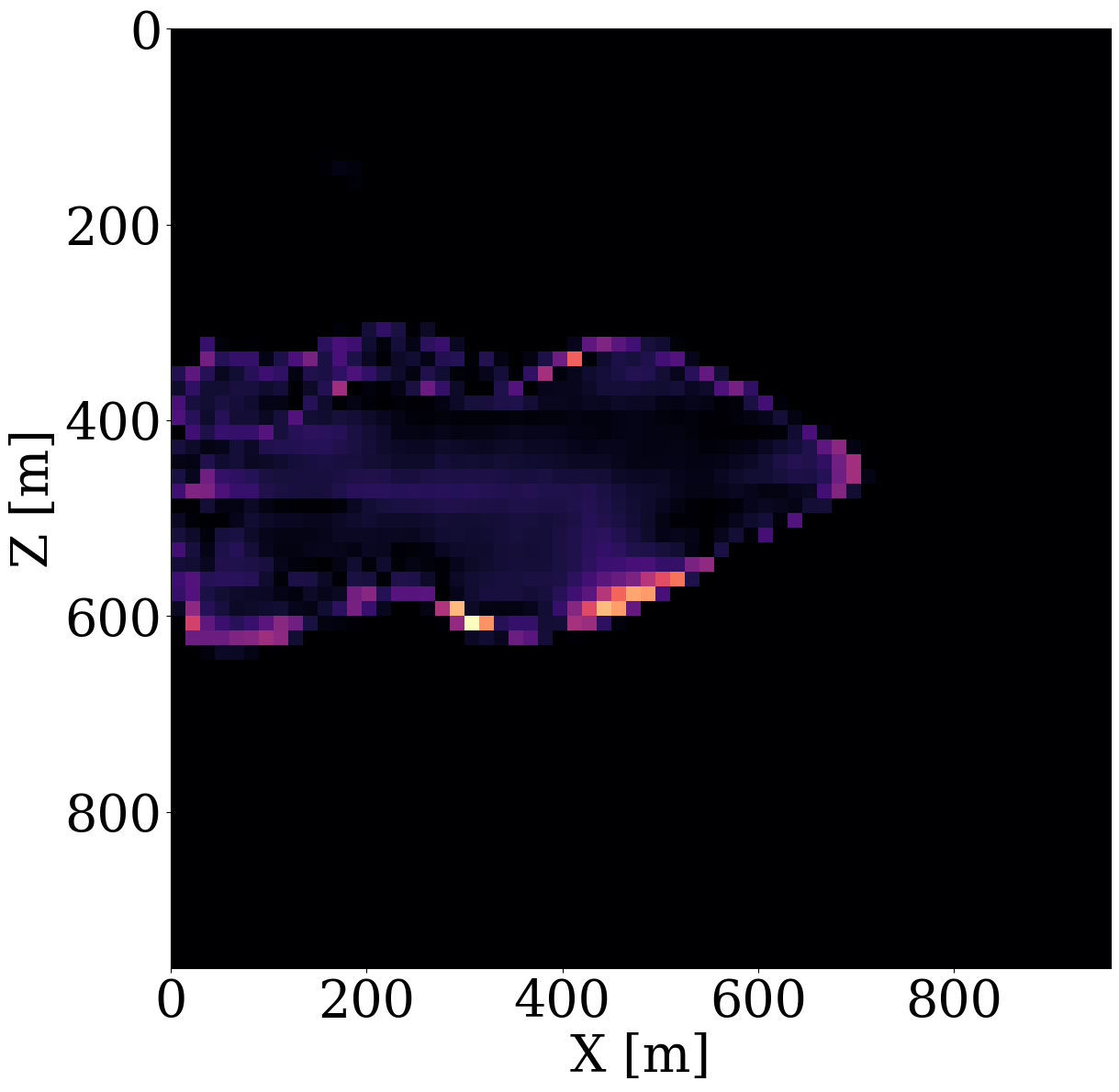
Inversion results obtained by solving the PDEs for the fluid flow during the inversion are shown in Figure 11 (a) and Figure 11 (c). As before, the inversions benefit majorly from adding the trained NF as a constraint. Remarkably, the end-to-end inversion results shown in Figure 11 (a), Figure 11 (c), and Figure 11 (d) are close to the results plotted in Figure 8 (a), Figure 8 (c), and Figure 8 (d), which was obtained with access to the CO2 saturation everywhere. This reaffirms the notion that time-lapse seismic can indeed provide useful spatial information away from the monitoring wells to estimate the reservoir permeability, which aligns with earlier observations by D. Li et al. (2020), Yin et al. (2022), and Louboutin, Yin, et al. (2023). Juxtaposing the results for the FNO surrogate without (Figure 11 (b)) and with the constraint (Figure 11 (d)) again underlines the importance of adding constraints especially in situations where the forward (wave) operator has a non-trivial nullspace. The presence of this nullspace has a detrimental affect on the unconstrained result obtained by the FNO. Contrary to solutions yielded by the PDE, trained FNOs offer little to no control on the feasibility of the solution, which explains the strong artifacts in Figure 11 (b). As we can see from Figure 11 (i), these artifacts are mainly due to the FNO-approximation errors that dominate and grow after a few iterations. Conversely, the errors for the constrained case remain more or less flatlined between \(7\%\) and \(8\%\). In contrast, using the trained NF as a learned constraint yields better recovery where the errors are minor within the plume region and mostly live on the edges, shown in the second row of Figure 11.
Jointly inverting time-lapse seismic data and well measurements
Finally, we consider the most preferred scenario for GCS monitoring, where multiple modalities of data are jointly inverted for the reservoir permeability (Huang 2022; M. Liu et al. 2023). In our experiment, we consider to jointly invert time-lapse seismic data and well measurements by minimizing the following objective function: \[ \underset{\mathbf{z}}{\operatorname{minimize}} \quad \|\mathbf{d}_{\mathrm{s}} - \mathcal{F}\circ\mathcal{R}\circ\mathcal{S}_{\boldsymbol\theta^\ast}\circ\mathcal{G}_{\mathbf{w}^\ast}(\mathbf{z})\|_2^2 + \lambda \|\mathbf{d}_{\mathrm{w}}-\mathbf{M}\circ\mathcal{S}_{\boldsymbol\theta^\ast}\circ\mathcal{G}_{\mathbf{w}^\ast}(\mathbf{z})\|_2^2 \quad\text{subject to}\quad\|\mathbf{z}\|_2\leq \tau. \tag{10}\]
This objective function includes both the time-lapse seismic data misfit from Equation 9 and the time-lapse well measurement misfit from Equation 8 with a balancing term \(\lambda\). While better choices can be made, we select this \(\lambda\) in our numerical experiment to be \(10\), so that the magnitudes of the two terms are relatively the same. The inversion results and differences from the unseen ground truth permeability are shown in Figure 12, where we again observe large artifacts for the recovery when FNO surrogate is inverted without NF constraints. This behavior is confirmed by the plot for the FNO error curve as a function of the number of iterations. This error finally reaches a value over \(15\%\).


We report quantitative measures for the permeability inversions for all optimization methods and different types of observed data in Table 1 for the signal-to-noise ratios (S/Ns) and the structural similarity index measure (SSIM, Wang et al. 2004). To avoid undue influence of the null space for the permeability, we only calculate the S/N and SSIM values based on the parts of the models that are touched by CO2 plume. From these values, following observations can be made. First, the NF-constrained permeability inversion are superior in both S/Ns and SSIMs, which demonstrates the efficacy of the learned constraint. Second, by virtue of this NF constraint, the results yielded by either the PDE solver or by the FNO surrogate produce very similar S/Ns and SSIMs. This behavior reaffirms that the trained FNO behavior is similar to the behavior yielded by PDE solver when its inputs remain in-distribution, which is controlled by the NF constraints.
| Inversion method | Well measurement | Time-lapse seismic | Both |
|---|---|---|---|
| Unconstrained inversion with PDE solvers | 9.34 dB / 0.67 | 10.50 dB / 0.73 | 10.70 dB / 0.73 |
| Unconstrained inversion with FNO surrogates | 9.64 dB / 0.68 | 11.94 dB / 0.72 | 11.98 dB / 0.72 |
| Constrained inversion with PDE solvers | 12.2 dB / 0.77 | 14.18 dB / 0.80 | 15.20 dB / 0.85 |
| Constrained inversion with FNO surrogates | 11.06 dB / 0.74 | 14.16 dB / 0.81 | 14.92 dB / 0.83 |
CO2 plume estimation and forecast
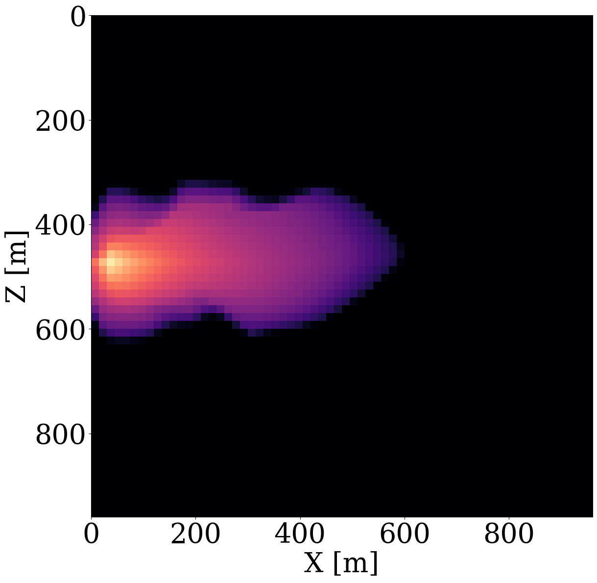
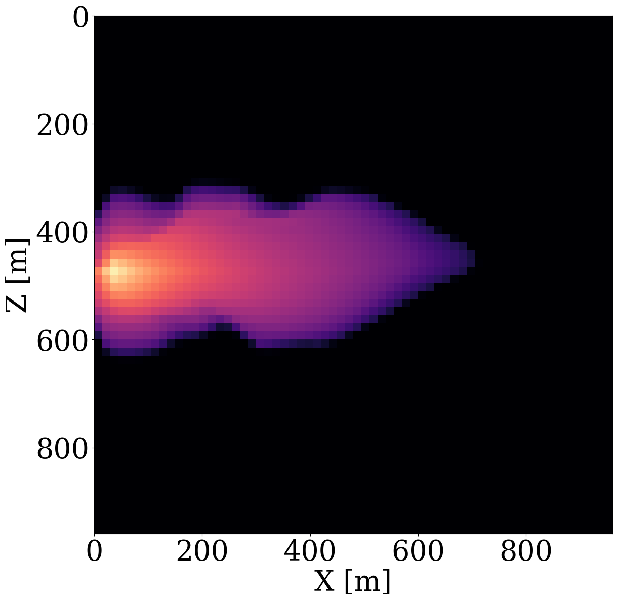
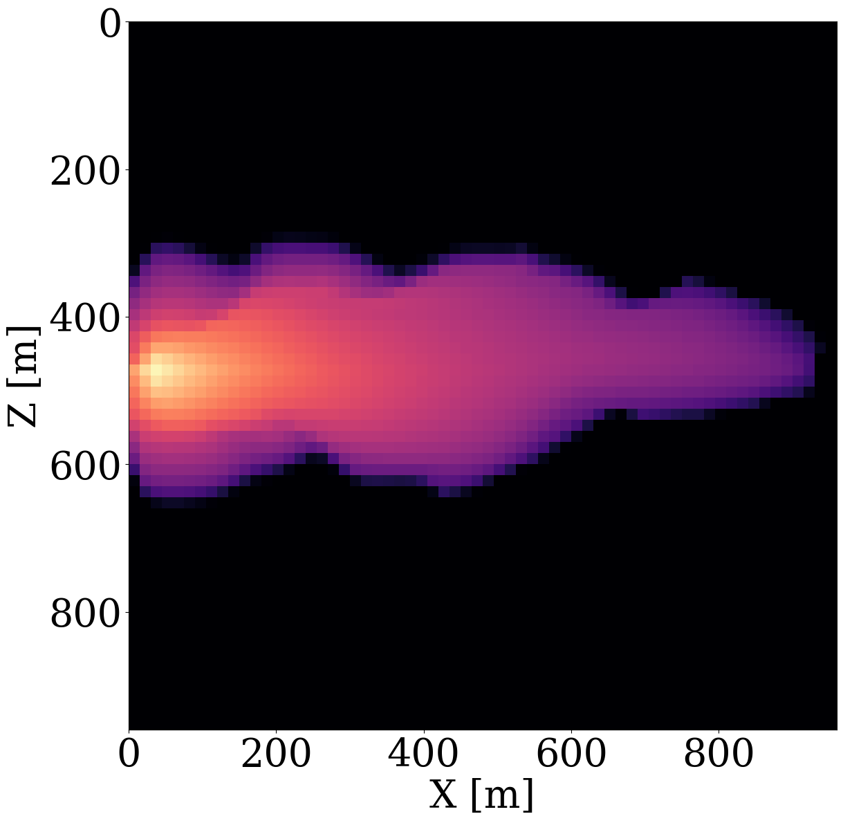
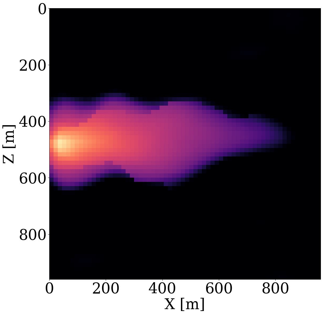
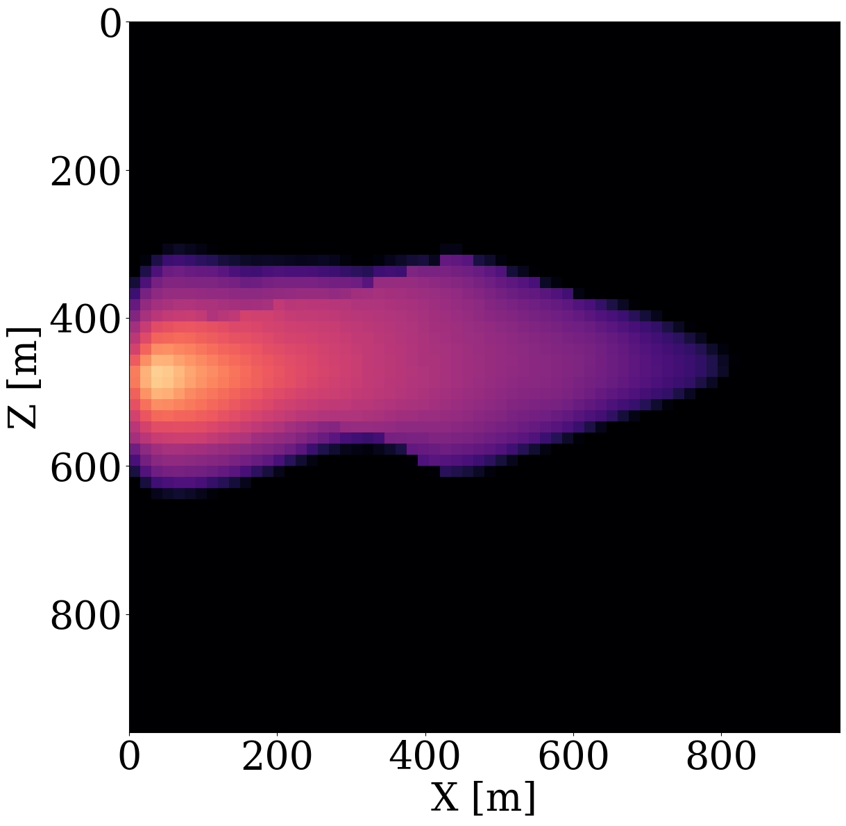
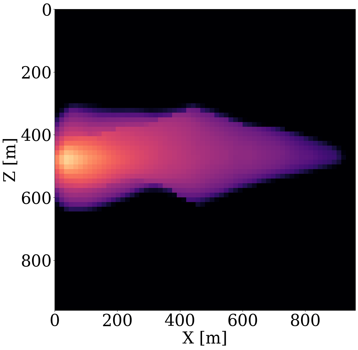
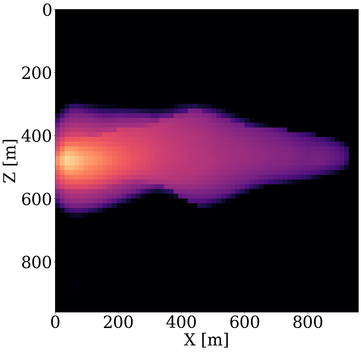
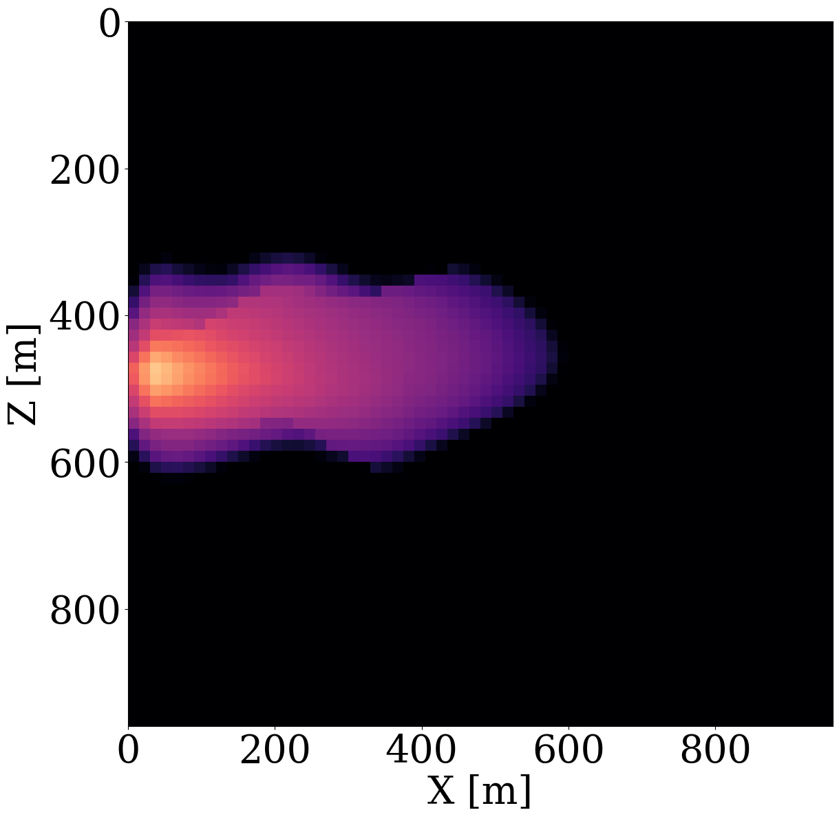
While end-to-end permeability inversion from time-lapse data provides novel access to this important fluid-flow property, the real interest in monitoring GCS lies in determining where CO2 plumes are and will be in the foreseeable future, say of 100 and 200 days ahead. To demonstrate the value of the proposed surrogates and of the use of time-lapse seismic data, as opposed to time-lapse saturation data measured at the wells only, we in Figure 7 juxtapose CO2 predictions obtained from fluid-flow simulations based on the inverted permeabilities in situations where either well data is available (first row), or where time-lapse seismic data is available (second row), or where both data modalities are available (third row). These results are achieved by first inverting for permeabilities using FNO surrogates and NF constraints, followed by running the fluid-flow simulations for additional time steps given the inverted permeabilities yielded by well-only (Figure 9 (d)), time-lapse data (Figure 11 (d)), and both (Figure 12 (d)). From these plots, we draw the following two conclusion. First, the predicted CO2 plumes estimated from seismic data are significantly more accurate than those obtained by inverting time-lapse saturations measured at the wells only. As expected, there are large errors in the regions away from the wells for the CO2 plumes estimated from wells shown in the fourth row of Figure 13. Second, thanks to the NF-constraint, the CO2 predictions obtained with the computationally beneficial surrogate approximation remain close to the ground truth CO2 plume plotted in the first row of Figure 7, with only minor artifacts at the edges. Third, using both seismic data and well measurements produces CO2 plume predictions with the smallest errors, while the uplift of well measurements on top of seismic observations is modest (comparing the second and the third rows of Figure 13). Finally, while the CO2 plume estimates for the past (monitored) vintages (i.e. first three columns of the third row of Figure 13) are accurate, the near-future forecasts without time-lapse well or seismic data (i.e. last two columns of the third row of Figure 13) could be less accurate. This is because the right-hand side and the bottom of the permeability model are not touched yet by the CO2 plume during the first 600 days. As a result, the error on the permeability recovery on the right-hand side leads to the slightly larger errors on the CO2 plume forecast. Overall, these CO2 forecasts for the future 100 and 200 days match the general trend of the CO2 plume without any observed data despite minor errors. A continuous monitoring system, where multiple modalities of data are being acquired and inverted throughout the GCS project, could allow for updating the reservoir permeability and forecasting the CO2 plume consistently.


Analysis of computational gains
FNOs, and deep neural surrogates in general, have the potential to be orders of magnitude faster than conventional PDE solvers (Z. Li et al. 2020), and this speed-up is generally problem-dependent. In our numerical experiments, the PDE solver from Jutul.jl (Møyner et al. 2023; Møyner, Bruer, and Yin 2023; Yin, Bruer, and Louboutin 2023) currently only supports CPUs and we find an average runtime for both the forward and gradient on the \(64 \times 64\) model to be 10.6 seconds on average on an 8-core Intel(R) Xeon(R) W-2245 CPU. The trained FNO, implemented using modules from Flux.jl (Innes 2018), takes 16.4 milliseconds on average for both the forward and gradient. This means that the trained FNO in our case provides \(646\times\) speed up compared to conventional PDE solvers. The training of FNO takes about 4 hours on an NVIDIA T1000 8GB GPU. Given these numbers, we can calculate the break-even point — i.e., the point where using FNO surrogate becomes cheaper in terms of the overall runtime, by the following formula:
\[ \textrm{breakeven} = \frac{\textrm{generating training set time} + \textrm{training time}}{\textrm{PDE solver runtime}-\textrm{FNO runtime}} \approx 3364. \tag{11}\]
This means that after 3364 calls to the forward simulator and its gradients, the computational savings gained from using the FNO surrogate evaluations during the inversion process balances out the initial upfront costs. These upfront costs include the generation of the training dataset and the training of the FNO. Therefore, after this break-even point of 3364 calls, the use of the FNO surrogate becomes more cost-effective compared to the conventional PDE solver. Because the trained FNO has the potential to generalize to different kinds of inversion problems, and potentially also different GCS sites, 3364 calls is justifiable in practice. However, we acknowledge that a more detailed analysis on a more realistic 4D scale problem will be necessary to understand the potential computational gains and tradeoffs of the proposed methodology. For details on a high-performance computing parallel implementation of FNOs, we refer to Grady et al. (2023) who also conducted a realistic performance on large-scale 4D multiphase fluid-flow problems. Even in cases where the computational advances are perhaps challenging to justify, the use of FNOs has the additional benefit by providing access to the gradient with respect to model parameters (i.e. permeability) through automatic differentiation. This feature is important since it is an enabler for inversion problems that involve complex PDE solvers for which gradients are often not readily available, e.g. Gross and Mazuyer (2021). By training FNOs on input-output pairs, “gradient-free” gradient-based inversion is made possible in situations where the simulator does not support gradients.
Discussion and conclusions
Monitoring of geological carbon storage is challenging because of excessive computational needs and demands on data collection by drilling monitor wells or by collecting time-lapse seismic data. To offset the high computational costs of solving multiphase flow equations and to improve permeability inversions from possibly multimodal time-lapse data, we introduce the usage of trained Fourier neural operators (FNOs) that act as surrogates for the fluid-flow simulations. We propose to do this in combination with trained normalizing flows (NFs), which serve as regularizers to keep the inversion and the accuracy of the FNOs in check. Since the computational expense of FNO’s online evaluation is negligible compared to numerically expensive partial differential equation solves, FNOs only incur upfront offline training costs. While this obviously presents a major advantage, the approximation accuracy of FNOs is, unfortunately, only guaranteed when its argument, the permeability, is in distribution—i.e., is drawn from the same distribution as the FNO was trained on. This creates a problem because there is, thanks to the non-trivial null space of permeability inversion, no guarantee the model iterates remain in-distribution. Quite the opposite, our numerical examples show that these iterates typically move out-of-distribution during the (early) iterations. This results in large errors in the FNO and in rather poor inversion results for the permeability.
To overcome this out-of-distribution dillema for the model iterates during permeability inversion with FNOs, we propose adding learned constraints, which ensure that model iterates remain in-distribution during the inversion. We accomplish this by training a NF on the same training set for the permeability used to train the FNO. After training, the NF is capable of generating in-distribution samples for the permeability from random realizations of standard Gaussian noise in the latent space. We employ this learned ability by parameterizing the unknown permeability in the latent space, which offers additional control on whether the model iterates remain in-distribution during the inversion. After establishing that out-of-distribution permeability models can be mapped to in-distribution models by restricting the \(\ell_2\)-norm of their latent representation, we introduce permeability inversion as a constrained optimization problem where the data misfit is minimized subject to a constraint on the \(\ell_2\)-norm of the latent space. Compared to adding pretrained NFs as priors via additative penalty terms, use of constraints ensures that model iterates remain at all times in-distribution. We show that this holds as long as the size of constraint set does not exceed the size of the \(\ell_2\)-norm ball of the standard normal distribution. As a result, we arrive at a computationally efficient continuation scheme, known as a homotopy, during which the \(\ell_2\)-norm constraint is relaxed slowly, so the data misfit objectives can be minimized while the model iterates remain in distribution.
By means of a series of carefully designed numerical experiments, we were able to establish the advocasy of combining learned surrogates and constraints, yielding solutions to permeability inversion problems that are close to solutions yielded by costly PDE-based methods. The examples also clearly show the advantages of working with gradually relaxed constraints where model iterates remain at all times in distribution with the additional joint benefit of slowly building up the model while bringing down the data misfit, an approach known to mitgate the effects of local minima (Peters and Herrmann 2017; Esser et al. 2018; Peters, Smithyman, and Herrmann 2019). Consequently, the quality of all time-lapse inversions improved significantly without requiring information that goes beyond having access to the training set of permeability models.
While we applied the proposed method to gradient-based iterative inversion, a similar approach can be used for other types of inversion methods, including inference with Markov chain Monte Carlo methods for uncertainty quantification (Lan, Li, and Shahbaba 2022). We also envisage extensions of the proposed method to other physics-based inverse problems (Heidenreich et al. 2014; Yang et al. 2023) and simulation-based inference problems (Cranmer, Brehmer, and Louppe 2020), where numerical simulations often form the computational bottleneck.
Despite the encouraging results from the numerical experiments, the presented approach leaves room for improvements, which we will leave for future work. For instance, the gradient with respect to the model parameters (permeability) derived from the neural surrogate is not guaranteed to be accurate—e.g. close to the gradient yielded by the adjoint-state method. As recent work by O’Leary-Roseberry et al. (2022) has shown, this potential source of error can be addressed by training neural surrogates on the simulator’s gradient with respect to the model parameters, provided it is available. Unfortunately, deriving gradients of complex HPC implementatons of numerical PDE solvers is often extremely challenging, explaining why this information is often not available. Because our method solely relies on gradients of the surrogate, which are readily available through algorithmic differentiation, we only need access to numerical PDE solvers available in legacy codes. While this approach may go at the expense of some accuracy, this feature offers a distinct practical advantage. However, as with many other machine learning approaches, our learned methods may also suffer from time-lapse observations that are out-of-distribution—i.e., produced by a permeability model that is out-of-distribution. While this is a common problem in data-driven methods, recent developments (Siahkoohi et al. 2023a) may remedy this problem by applying latent space corrections, a solution that is amenable to our approach. On the other hand, expanding the latent space’s \(\ell_2\) norm ball during inversion would allow NFs to generate any out-of-distribution model parameter. However, in that case the accuracy of the learned surrogate is not guaranteed. For such cases, transitioning from the learned surrogate to the numerical solver during later iterations may be advantageous and merits further study. The choice for the size of the \(\ell_2\)-norm ball at the beginning and at the end can also be further investigated (Aster, Borchers, and Thurber 2018).
While our paper primarily presents a proof of concept through a relatively small 2D experiment, our inversion strategy is designed to scale to large-scale 3D problems. NFs, with their inherent memory efficiency due to invertibility, are already primed for extension to 3D problems. For the learned surrogates, Grady et al. (2023) showcases model-parallel FNOs, demonstrating success in simulating 4D multiphase flow physics of over 2.6 billon variables. By combining these strengths, we are optimistic scaling this inversion strategy to 3D.
To end on a positive note and forward looking note, we argue that the presented approach makes a strong case for the inversion of multimodal data, consisting of time-lapse well and seismic data. While inversions from time-lapse saturation data collected from wells are feasible and fall within the realm of reservoir engineering, their performance, as expected, degrades away from the well. We argue that adding active-source seismic provides essential fill-in away from the wells. As such, it did not come to our surprise that joint inversion of multimodal data resulted in the best permeability estimates. From our perspective, our successfull combination of these often disjoint data modalities holds future promise when addressing challenges that come with monitoring and control of geological carbon storage and enhanced geothermal systems.
Availability of data and materials
The scripts to reproduce the experiments are available on the SLIM GitHub page https://github.com/slimgroup/FNO-NF.jl.
Abbreviations
FNO: Fourier neural operator
GCS: geological carbon storage
NF: normalizing flow
PDE: partial differential equations
Acknowledgements
The authors would like to thank Philipp A. Witte at Microsoft, Ali Siahkoohi at Rice University, and Olav Møyner at SINTEF for constructive discussions. The authors gratefully acknowledge the contribution of OpenAI’s ChatGPT for refining sentence structure and enhancing the overall readability of this manuscript.
Funding
This research was carried out with the support of Georgia Research Alliance and partners of the ML4Seismic Center. This research was also supported in part by the US National Science Foundation grant OAC 2203821 and the Department of Energy grant No. DE-SC0021515.
Ethics declarations
Competing interests
The authors declare that they have no competing interests.