Learned coupled inversion for carbon sequestration monitoring and forecasting with Fourier neural operators

Summary

Seismic monitoring of carbon storage sequestration is a challenging problem involving both fluid-flow physics and wave physics. Additionally, monitoring usually requires the solvers for these physics to be coupled and differentiable to effectively invert for the subsurface properties of interest. To drastically reduce the computational cost, we introduce a learned coupled inversion framework based on the wave modeling operator, rock property conversion and a proxy fluid-flow simulator. We show that we can accurately use a Fourier neural operator as a proxy for the fluid-flow simulator for a fraction of the computational cost. We demonstrate the efficacy of our proposed method by means of a synthetic experiment. Finally, our framework is extended to carbon sequestration forecasting, where we effectively use the surrogate Fourier neural operator to forecast the CO₂ plume in the future at near-zero additional cost.

Introduction

Time-lapse seismic monitoring of CO₂ sequestration is one of the most commonly used technologies to monitor CO₂ dynamics in the Earth’s subsurface through multiple seismic surveys (vintages) (D. E. Lumley, 2001). Time-lapse seismic has been used by carbon capture and storage (CCS) practitioners at various storage sites (O. Eiken et al., 2000; R. Arts et al., 2003; A. Chadwick et al., 2010; PS Ringrose et al., 2013; Furre et al., 2017). The growth of the CO₂ plumes can be inferred by time-lapse seismic imaging (R. Arts et al., 2003; Ayeni and Biondi, 2010; Maria Kotsi, 2020; Yin et al., 2021) or by time-lapse full-waveform inversion (Queißer and Singh, 2013; D. Yang et al., 2016; M Kotsi et al., 2020). Unfortunately, plain subtractions of time-lapse seismic images or inversion results often contain unwanted artifacts due to noise or to differences in acquisition (Oghenekohwo and Herrmann, 2017a; Zhou and Lumley, 2021b), which can potentially corrupt the often rather subtle time-lapse differences due to changes in CO₂ concentration.

Over the years, several attempts have been made to mitigate this challenge by improving the repeatability of time-lapse seismic, including the forward and backward bootstrapping method (Asnaashari et al., 2015), the double-difference method (Watanabe et al., 2004; Denli and Huang, 2009; Z. Zhang and Huang, 2013; D. Yang et al., 2015), the central-difference method (Zhou and Lumley, 2021a), data assimilation via Kalman filtering (J. Y. Li et al., 2014; Eikrem et al., 2019; C. Huang and Zhu, 2020) and the joint recovery model (Oghenekohwo et al., 2017; Wason et al., 2017; Oghenekohwo and Herrmann, 2017b; Yin et al., 2021). While these methods resulted in improvements in repeatability of time-lapse seismic, they ignore the fact that the dynamics of CO₂ plumes, to the leading order, adhere to two-phase flow equations. Given physical properties of the two fluids (brine and supercritical CO₂) and the spatial porosity and permeability distributions, these fluid-flow equations are capable of predicting CO₂ concentration snapshots during and after CO₂ injection. By coupling these fluid-flow equations, via a rock physics model (the patchy saturation model (Avseth et al., 2010)), to the wave equation, D. Li et al. (2020) proposed an end-to-end inversion framework where time-lapse seismic surveys are jointly inverted to yield estimates for the spatial permeability distribution. Compared to the sequential inversion (Mohamed Hatab and MacBeth, 2021; M Hatab and MacBeth, 2021) and history matching workflows (Oliver et al., 2021), estimates of the CO₂ concentration in the coupled inversion are regularized by fluid-flow physics. Because coupled inversion (D. Li et al., 2020) makes use of the fluid-flow equations, it offers a framework capable of producing direct estimates for the permeability. The latter can be used to generate improved predictions for the behavior of CO₂ plumes. Despite the initially promising results by D. Li et al. (2020) on synthetic experiments, the downside of their proposed coupled framework is the increased complexity that comes with including partial differential equations (PDEs) for the fluid-flow as constraints. Aside from the need to compute sensitivities of solutions of the fluid-flow equations, solving these PDE can be computationally expensive (Settgast et al., 2018; Rasmussen et al., 2021).

To address this challenge, we propose to replace solvers for the fluid-flow PDEs by Fourier neural operators (FNOs, Z. Li et al., 2020). After training on a representative dataset, FNOs are capable of producing CO₂ plume snapshots quickly (Wen et al., 2021a; K. Zhang et al., 2022) while automatic differentiation (AD) gives us easy and fast access to the gradient with respect to the input. As such, trained FNOs can be considered as a data-driven surrogate for the computationally expensive fluid-flow simulations, making them a suitable candidate for the proposed coupled inversion framework that calls for multiple fluid-flow simulations including calculation of the gradient.

This extended abstract is organized as follows. First, we discuss the coupled inversion framework for seismic monitoring of geological carbon storage. Second, we introduce FNOs as surrogates for fluid-flow simulations. Next, we present the learned FNO-based coupled inversion framework where the fluid-flow solver is replaced by a pre-trained FNO. Finally, we verify the efficacy of the learned coupled inversion framework through a synthetic experiment. We further show that the trained FNO can forecast the growth of the CO₂ plume in the future with the inverted permeability model.

Coupled inversion framework

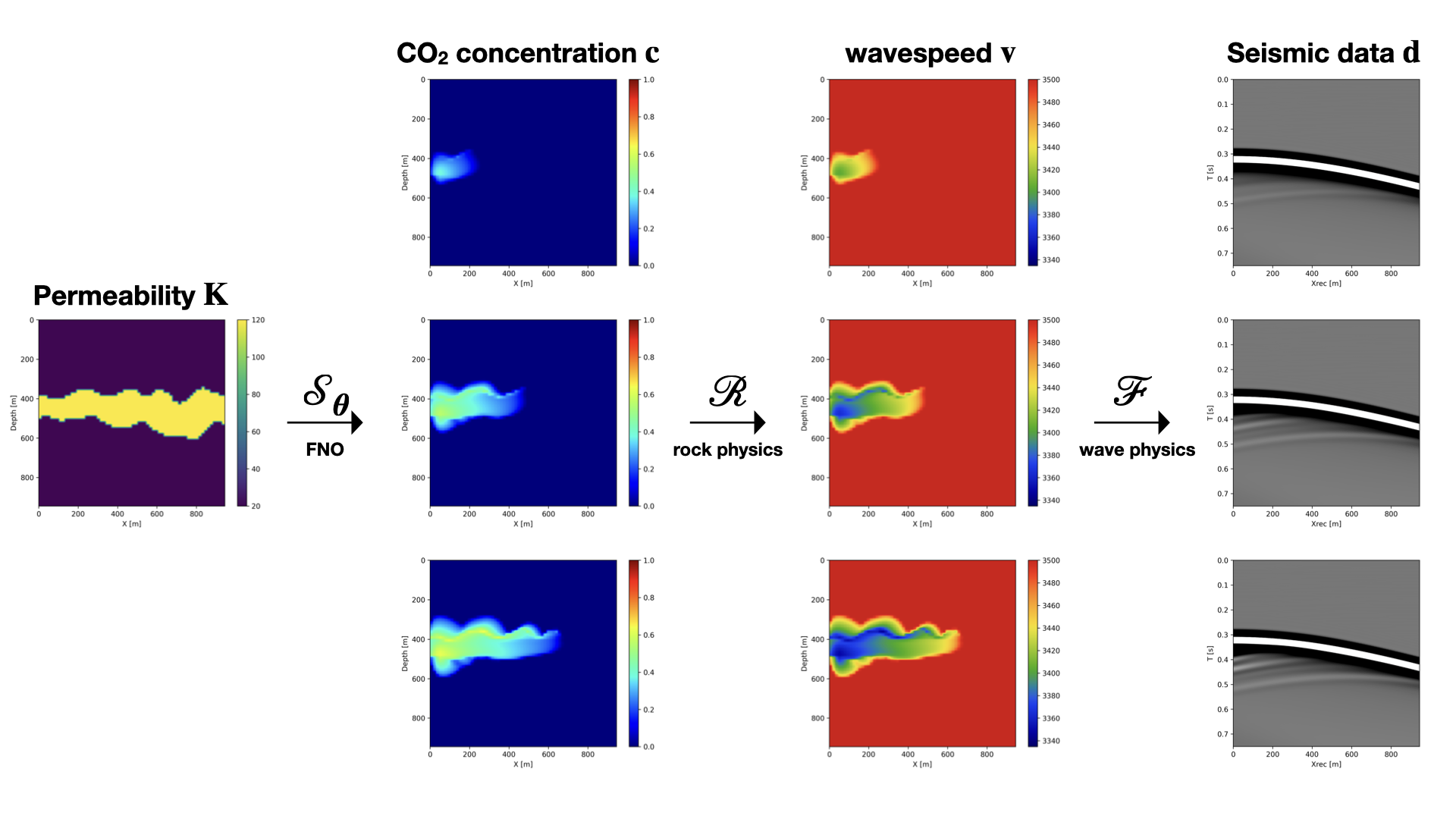
Our goal is to estimate the past, current, and future behavior of CO₂ plumes from available time-lapse seismic data. To achieve this goal, we consider the coupled inversion framework proposed by D. Li et al. (2020). In this framework, three types of physics are integrated, namely fluid-flow, rock, and wave physics. The CO₂ plume dynamics are modeled by two-phase flow equations (Pruess and Nordbotten, 2011), which we represent as the following mapping: \[ \begin{equation} \mathbf{K}\mapsto\mathbf{c}=\mathcal{S}(\mathbf{K})\quad\text{where} \quad \mathbf{c}=[\mathbf{c}_1,\mathbf{c}_2,\ldots,\mathbf{c}_{n_v}], \label{fluidflow} \end{equation} \] where the vectors \(\mathbf{c}_i,\,i=1\ldots n_v\) are the discretized CO₂ concentration snapshots for each vintage. In this mapping, \(\mathcal{S}\) represents two-phase flow simulations that given the permeability, \(\mathbf{K}\), models the CO₂ concentration as a spatial function over \(n_v\) consecutive times. Then, the patchy saturation model (Avseth et al., 2010) maps the \(n_v\) snapshots of the CO₂ concentration to seismic wavespeeds—i.e., we introduce for each vintage (\(i=1\ldots n_v\)) the following mapping: \[ \begin{equation} \mathbf{c}_i\mapsto\mathbf{v}_i = \mathcal{R}(\mathbf{c}_i) \quad \text{for} \quad i=1, 2, \ldots, n_v, \label{patchy} \end{equation} \] where \(\mathcal{R}\) represents the rock physics model and \(\mathbf{v}_i,\, i=1\cdots n_v\) the snapshots of the acoustic wavespeed. To connect these wavespeed snapshots to the seismic data vintages, we introduce the mapping: \[ \begin{equation} \mathbf{v}_i\mapsto\mathbf{d}_i = \mathcal{F}_i(\mathbf{v}_i) \quad \text{for} \quad i=1, 2, \ldots, n_v, \label{seismic} \end{equation} \] where \(\mathcal{F}_i\) is the wave modeling operator for vintage \(i\) that generates the corresponding seismic dataset \(\mathbf{d}_i\) given the velocity model \(\mathbf{v}_i\) (Tarantola, 1984; Virieux and Operto, 2009). To arrive at the end-to-end formulation linking multi-vintage seismic data to the permeability, we finally compose (denoted by the \(\circ\) symbol) these three mappings yielding the following minimization problem: \[ \begin{equation} \begin{split} \underset{\mathbf{K}}{\operatorname{minimize}} \quad \frac{1}{2}\|\mathcal{F}\circ\mathcal{R}\circ\mathcal{S}(\mathbf{K})-\mathbf{d}\|_2^2 \\ \text{where} \quad \mathbf{d}=[\mathbf{d}_1,\mathbf{d}_2,\ldots,\mathbf{d}_{n_v}], \end{split} \label{couple} \end{equation} \] where \(\mathbf{d}\) represents the \(n_v\) vintages of the time-lapse data. While the optimization problem \(\ref{couple}\) offers a unique formulation where time-lapse seismic data are linked to the permeability, its minimization is complex since it entails nested application of the adjoint-state method (Plessix, 2006) involving computationally expensive forward simulations of both wave and fluid-flow physics. To simplify the formulation and to drastically reduce computational cost of minimization problem \(\ref{couple}\), we propose to replace the fluid-flow solves by a trained FNO.

Fourier neural operators

There exists a growing literature on solving numerical PDEs via learned data-driven approaches involving neural networks (Lu et al., 2019; Raissi et al., 2019; Kochkov et al., 2021; Karniadakis et al., 2021). After incurring initial training costs, neural networks have been shown to to provide faster alternatives to numerical PDE simulations. Recently, FNOs (Z. Li et al., 2020, 2021) have emerged as a powerful technique to approximate the solution operator of parametric PDEs. After training, FNOs can generate approximation solutions of PDEs from the coefficients orders of magnitude faster than numerical solvers (Z. Li et al., 2020). This means that computational costs, which consist of generating training pairs coefficient (permeability \(\mathbf{K}\)) and solution (CO₂ concentration \(\mathbf{c}\)) and training the network, are sustained upfront. This front loading of computations leads to a drastic reduction in simulation time during the inversion—i.e., minimization of problem \(\ref{couple}\). We refer to the existing literature (Wen et al., 2021a; K. Zhang et al., 2022) for details on how to train FNOs to approximately map permeability models to the time evolution of CO₂ plumes. In this abstract, we assume to have \(\mathcal{S}_{\boldsymbol{\theta}}(\mathbf{K})\approx \mathcal{S}(\mathbf{K})\) for the permeability drawn from a certain distribution. Here, \(\mathcal{S}_{\boldsymbol{\theta}}(\cdot)\) denotes the approximate map, which depends on the learned FNO weights \({\boldsymbol{\theta}}\). Given an unseen spatial distribution for the permeability \(\mathbf{K}\), the trained FNO can instantaneously produce the time-dependant CO₂ concentration by forward evaluation of the FNO as \(\mathcal{S}_{\boldsymbol{\theta}}(\mathbf{K})\) (Z. Li et al., 2020; Wen et al., 2021a; K. Zhang et al., 2022). In addition, AD gives us access to the gradient with respect to FNO’s input (the permeability \(\mathbf{K}\)) that can be used for inversion. By virtue of these capabilities, the proposed approximation by FNOs can be used as a surrogate for the fluid-flow solver in the end-to-end formulation of problem \(\ref{couple}\).

Forecast via learned coupled inversion

While the end-to-end formulation (shown in Figure 1) provides access to estimates of the permeability, CO₂ plume forecasting (Wen et al., 2021b) is our main objective because they offer guarantees that the CO₂ plume is progressing as planned. To meet our goal of CO₂ plume forecasting, the proposed learned and coupled formulation offers several distinct advantages. First, the coupled formulation uses information from all collected time-lapse vintages to arrive at estimates for the permeability itself and past and current behavior of the CO₂ plume. The fact that the two-phase flow equations act as a regularizer leads to improved estimates for the CO₂ plume (D. Li et al., 2020). Second, the use of FNOs reduces the computational cost (Z. Li et al., 2020; Wen et al., 2021a), which potentially enables uncertainty quantification and risk management of the growth of the CO₂ plume in the future. Third, the coupled framework provides access to estimates for the permeability that can be used to forecast future behavior of CO₂ plumes. Given the estimated permeability model from the learned coupled inversion and an FNO trained on the time range of CCS projects, the current and future CO₂ concentration snapshots can all be generated by forward evaluation of the FNO. The forecast of CO₂ plume in the future can help the practitioners to detect potential failing scenarios in the early period of the CCS project, such as CO₂ leaking through fractures in the seal (Philip Ringrose, 2020).

Numerical experiments

By means of a synthetic case study, we validate the performance of our FNO-based learned coupled inversion framework to invert for the permeability from time-lapse seismic data. We then show that we can use the estimated permeability to forecast the evolution of the CO₂ plume in the future. We begin by describing how we train the FNO to learn the two-phase flow physics.

Training setup

We create \(1000\) pairs of permeability and time evolution of CO₂ concentration to form the training set. The size of the permeability is \(64 \times 64\) with a grid spacing of \(15\,\mathrm{m}\) in both vertical and horizontal directions. Each permeability model is \(20\,\) millidarcies (md) everywhere except for a high permeability channel with \(120\,\mathrm{md}\) in the central area of the model, of which the random curving boundaries are generated by a Gaussian process (Bishop and Nasrabadi, 2006). An example of the permeability model in shown in Figure 2a. For fluid-flow simulation, we add an injection well that injects supercritical CO₂ (with density \(501.9\,\mathrm{kg}/\mathrm{m}^3\)) on the left-hand side of the model, and a production well that produces brine (with density \(1053.0\,\mathrm{kg}/\mathrm{m}^3\)) on the right-hand side of the model. We assume the porosity of the reservoir is fixed to \(25\%\) homogeneously. The time evolution of the CO₂ concentration is modeled with FwiFlow.jl (D. Li et al., 2020) over a period of \(1000\) days with a time step of \(20\) days. This numerical simulation creates \(51\) snapshots in total for each permeability model. We form the training dataset, where each sample is a pair of the permeability model and corresponding \(51\) snapshots of CO₂ concentration. We train an FNO that maps the input permeability \(\mathbf{K}(x,z,t)\) to the output CO₂ concentration \(\mathbf{c}(x,z,t)\). We follow the original implementation of FNOs https://github.com/zongyi-li/fourier_neural_operator (Z. Li et al., 2020) and re-implement the FNO in Julia in order to integrate with other software modules in the learned coupled inversion framework.

Learned coupled inversion from time-lapse seismic data

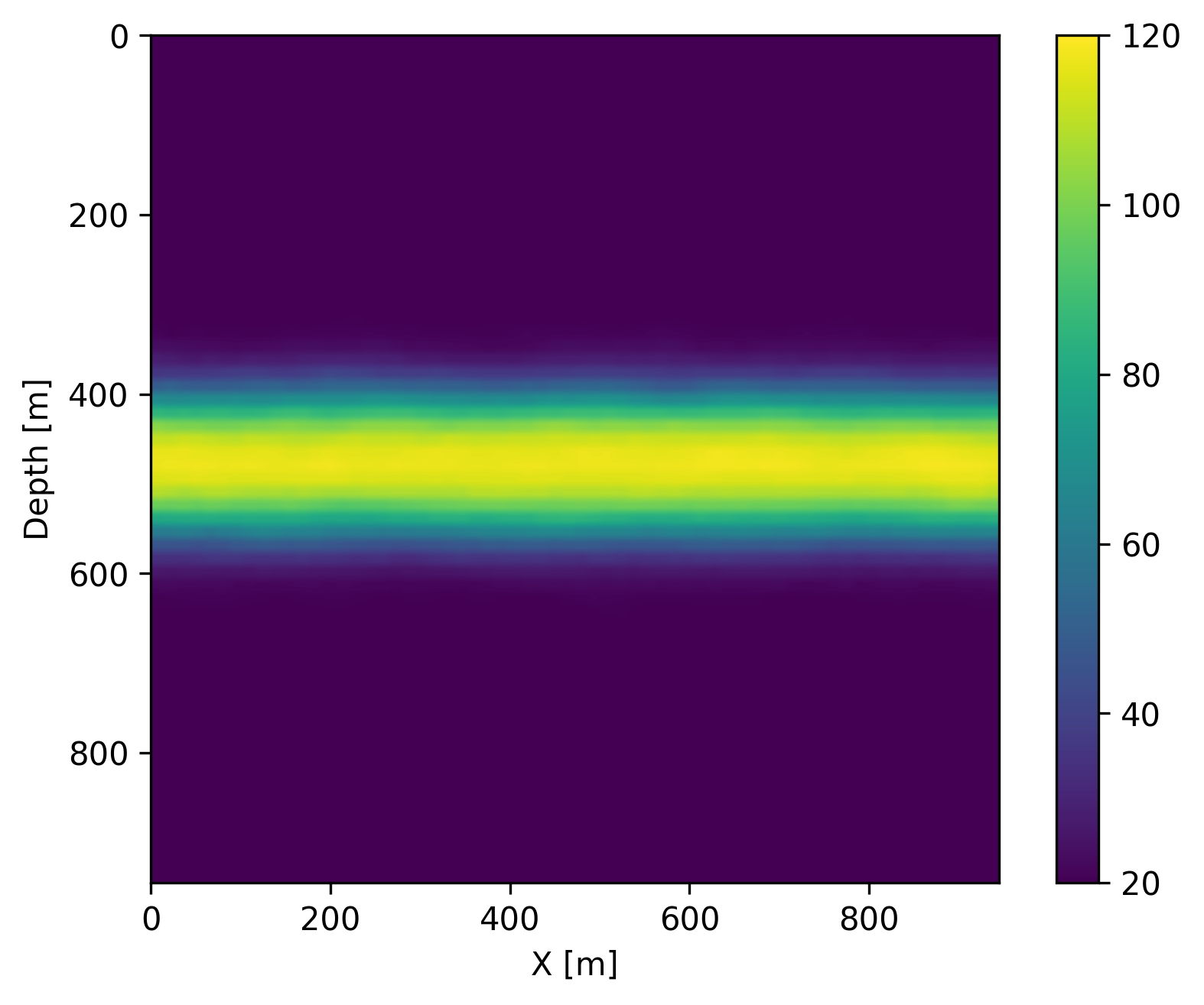
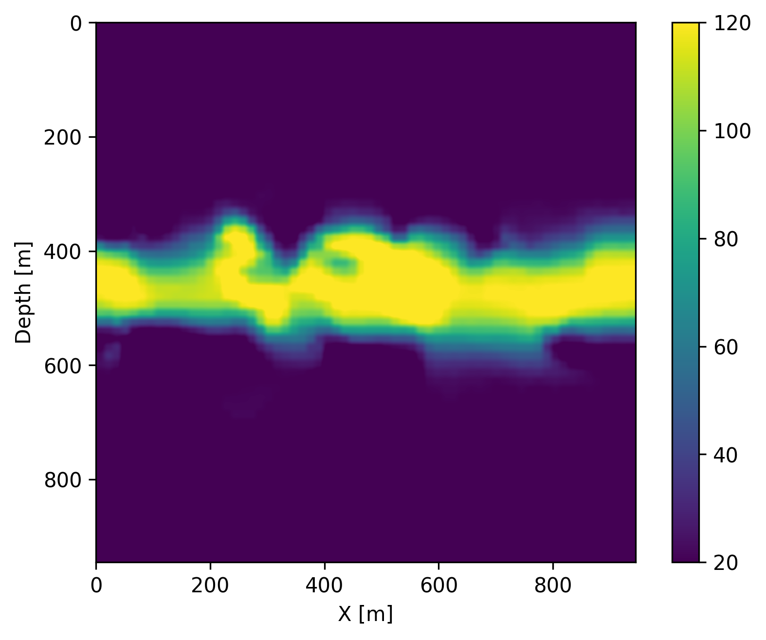
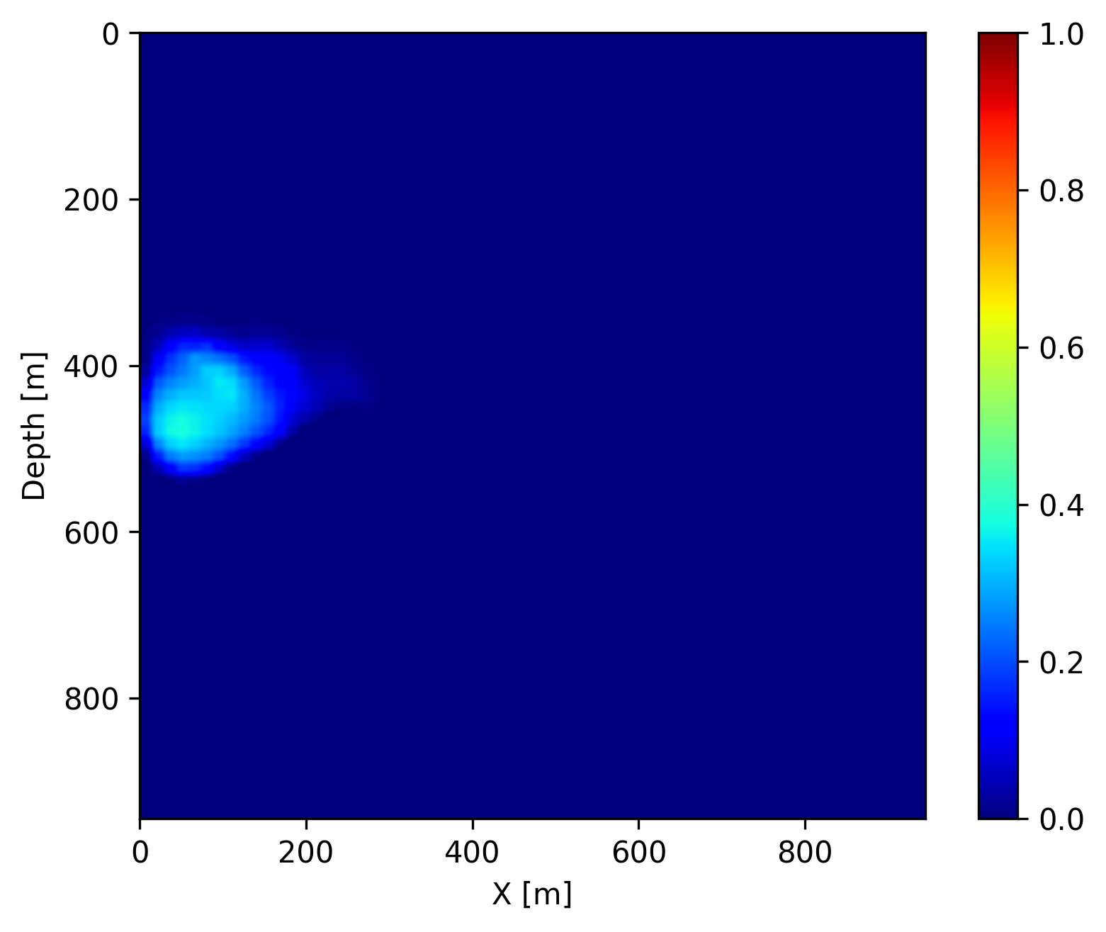
After training, we show the performance of the learned coupled inversion framework described in Figure 1. During testing, we draw an unseen permeability sample, shown in Figure 2a, and generate \(11\) early snapshots of CO₂ concentration at every \(40\)th day using the numerical solvers. The snapshots at day \(40\), \(160\) and \(280\) are shown in Figure 3d, 3e, 3f, respectively. Since these are the early snapshots, the CO₂ plume does not reach the entire high permeability channel from the left to the right. We then convert these CO₂ concentration snapshots to the time-varying velocity models via the patchy saturation model (Avseth et al., 2010), and generate \(11\) cross-well seismic surveys on these \(11\) velocity models. The wave physics is modeled with JUDI.jl (P. A. Witte et al., 2019; Louboutin et al., 2022), which uses the highly-optimized matrix-free wave propagators of Devito (Louboutin et al., 2019; Luporini et al., 2020, 2022). Each seismic survey contains \(32\) active sources in a borehole on the left-hand side of the model, and \(960\) receivers in a borehole on the right-hand side of the model. We then invert for the permeability from the time-lapse seismic data via the learned coupled inversion framework in Figure 1. We start our initial guess as an average of the samples in the training set (a blurred channel shown in Figure 2b), and iteratively solve for the permeability by projected gradient descent with a box constraint on the permeability between \(10\,\mathrm{md}\) and \(130\,\mathrm{md}\). At each iteration, we compute the seismic data misfit for only four shot records in each time-lapse survey. This reduces the cost of wave physics as only one eighth of the shot records are used during the forward and gradient evaluation (X. Li et al., 2012; Leeuwen and Herrmann, 2013). We use the backtracking linear search algorithm (Stanimirović and Miladinović, 2010) to choose the step length accordingly. We use SetIntersectionProjection.jl (Peters and Herrmann, 2019; Peters et al., 2021) for box constraint projection. After \(120\) iterations (\(15\) data passes on the entire time-lapse dataset), the inverted permeability is shown in Figure 2c. Since the CO₂ plume grows mostly at the left part of the channel (near the injection well) in these early snapshots, some part of the permeability model is in the null space thus difficult to recover exactly. However, we can see that the learned coupled inversion is able to approximately estimate the high permeability channel and to delineate curvatures especially at the upper boundary. Next, we demonstrate that this estimate is already remarkably accurate to recover the shape of the CO₂ plume and forecast the growth of the CO₂ plume in the future.

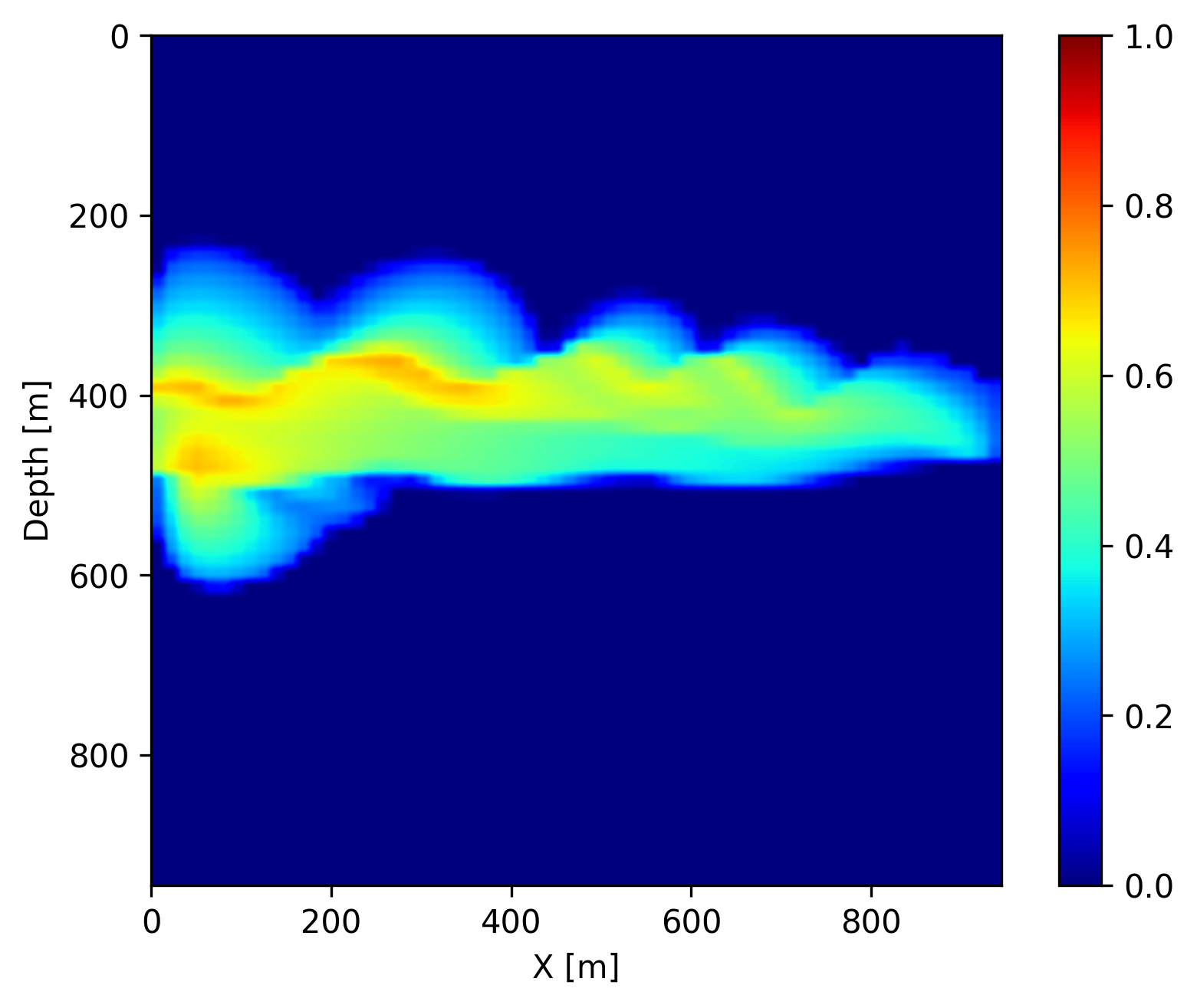
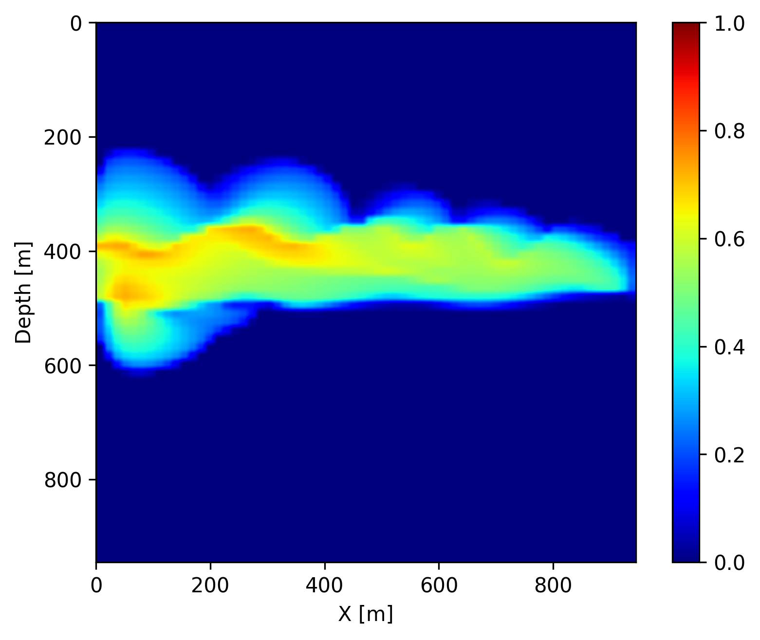
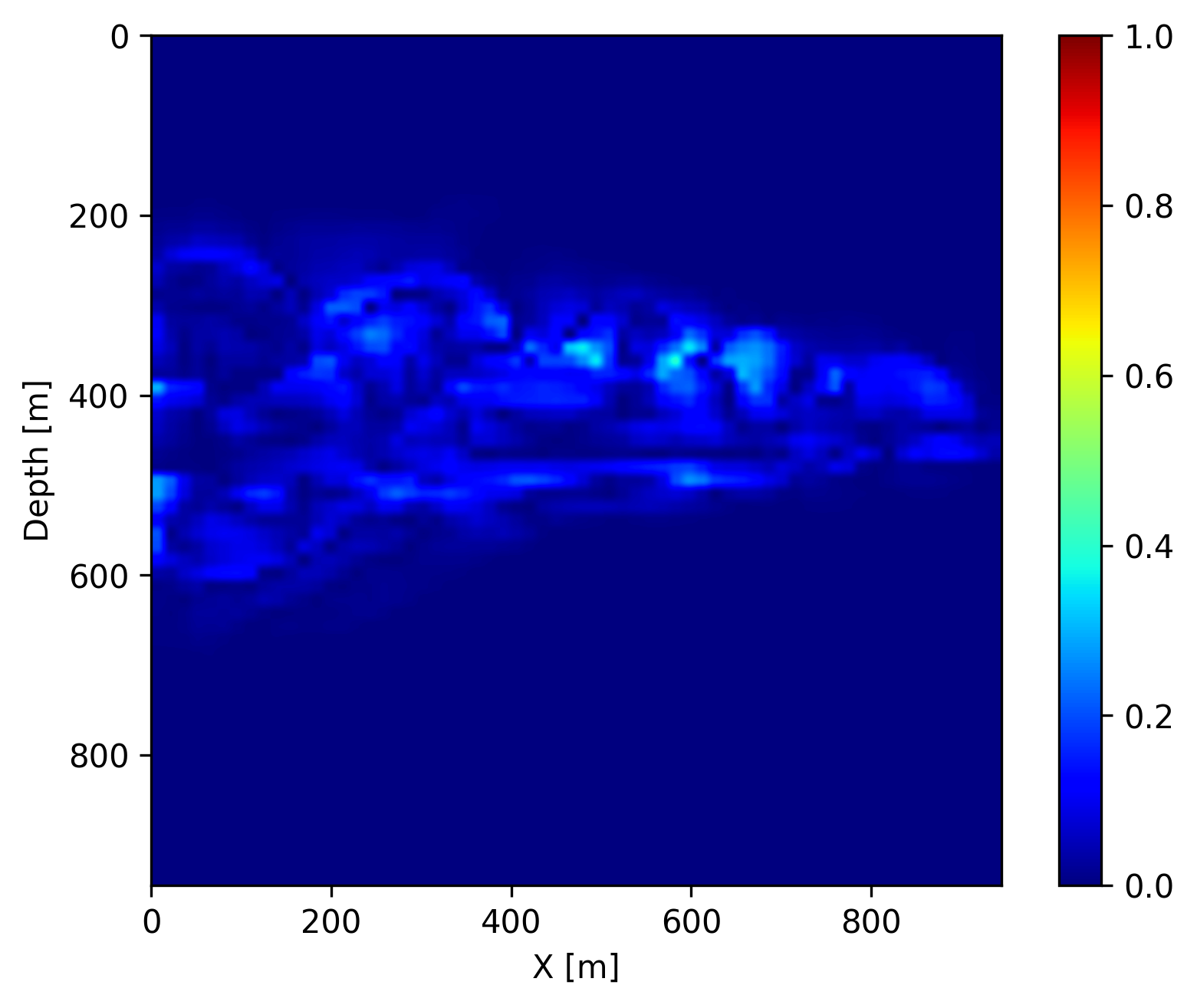
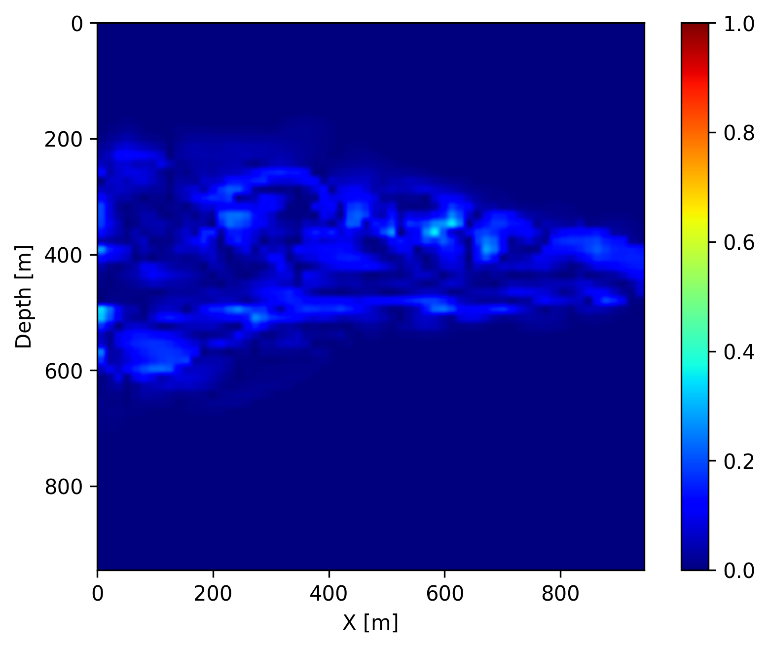
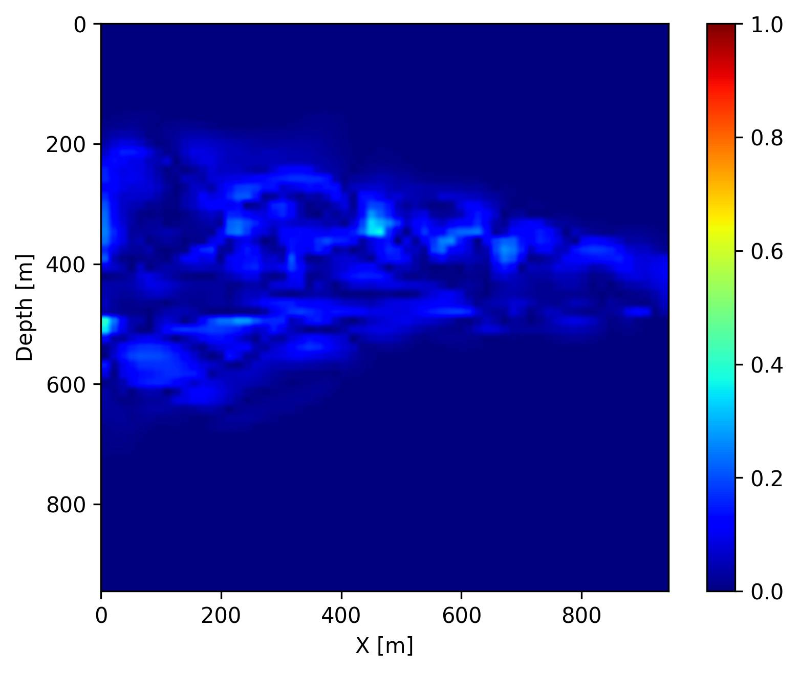
In addition to recovering the permeability, we are interested in CO₂ concentration recovery as it indicates the growing progress of the CO₂ plume. In Figure 3, we show the recovered CO₂ concentration snapshots at day \(40\), \(160\) and \(280\), which are acquired by a forward evaluation of FNO on the inverted permeability. We juxtapose the recovered concentrations snapshots with the ground truth and the differences for easy visualization. We observe that our predicted CO₂ concentration snapshots fit the ground truth accurately with very few artifacts near the boundaries of the CO₂ plume. This demonstrates that the proposed learned coupled inversion framework can be used successfully for carbon storage monitoring.

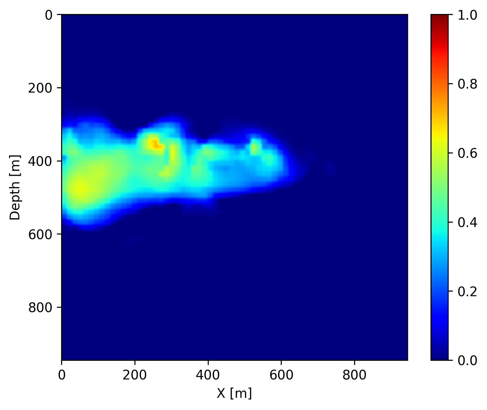
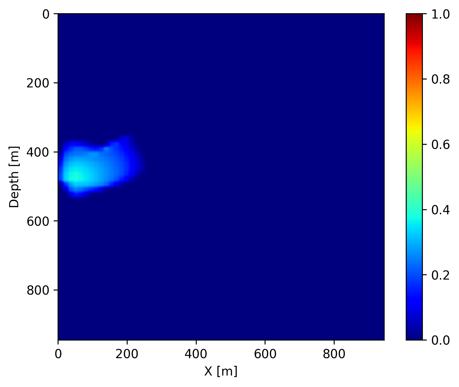
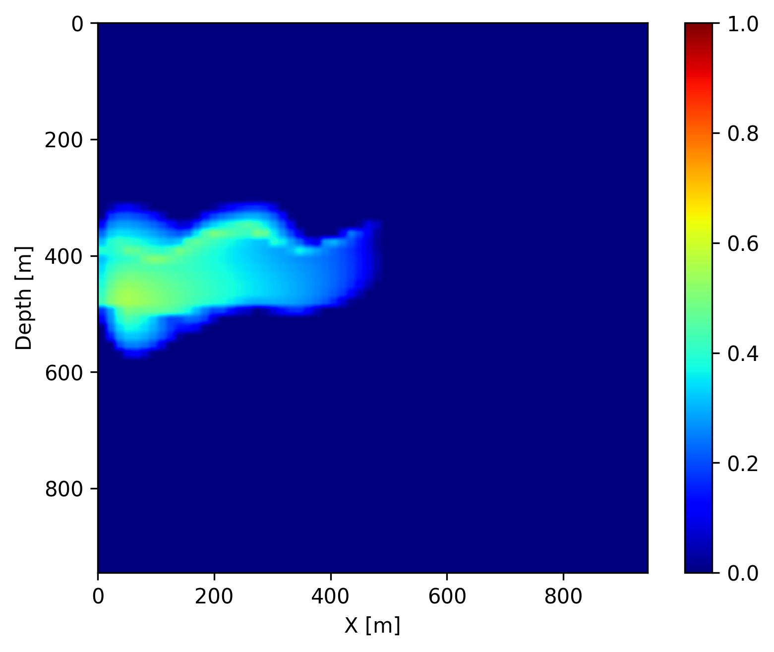
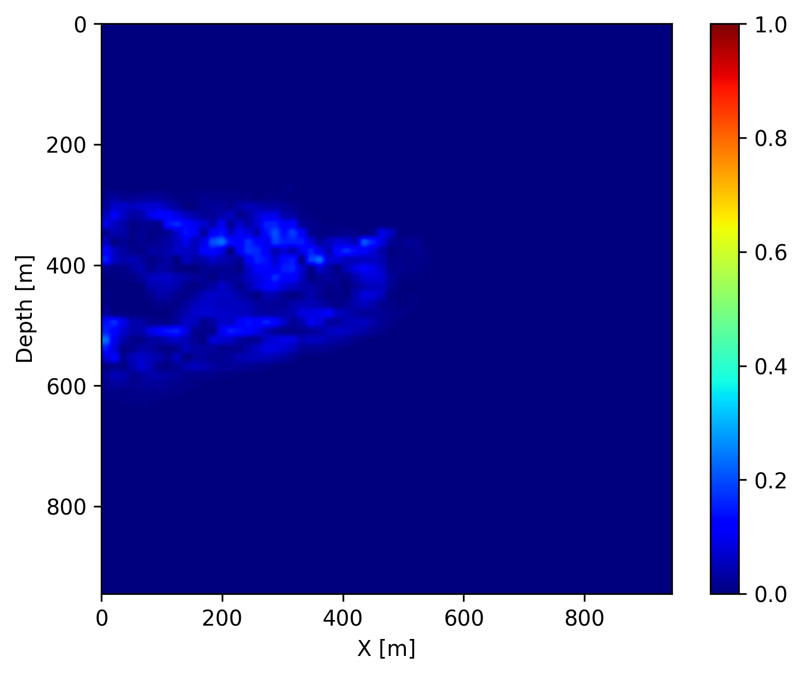
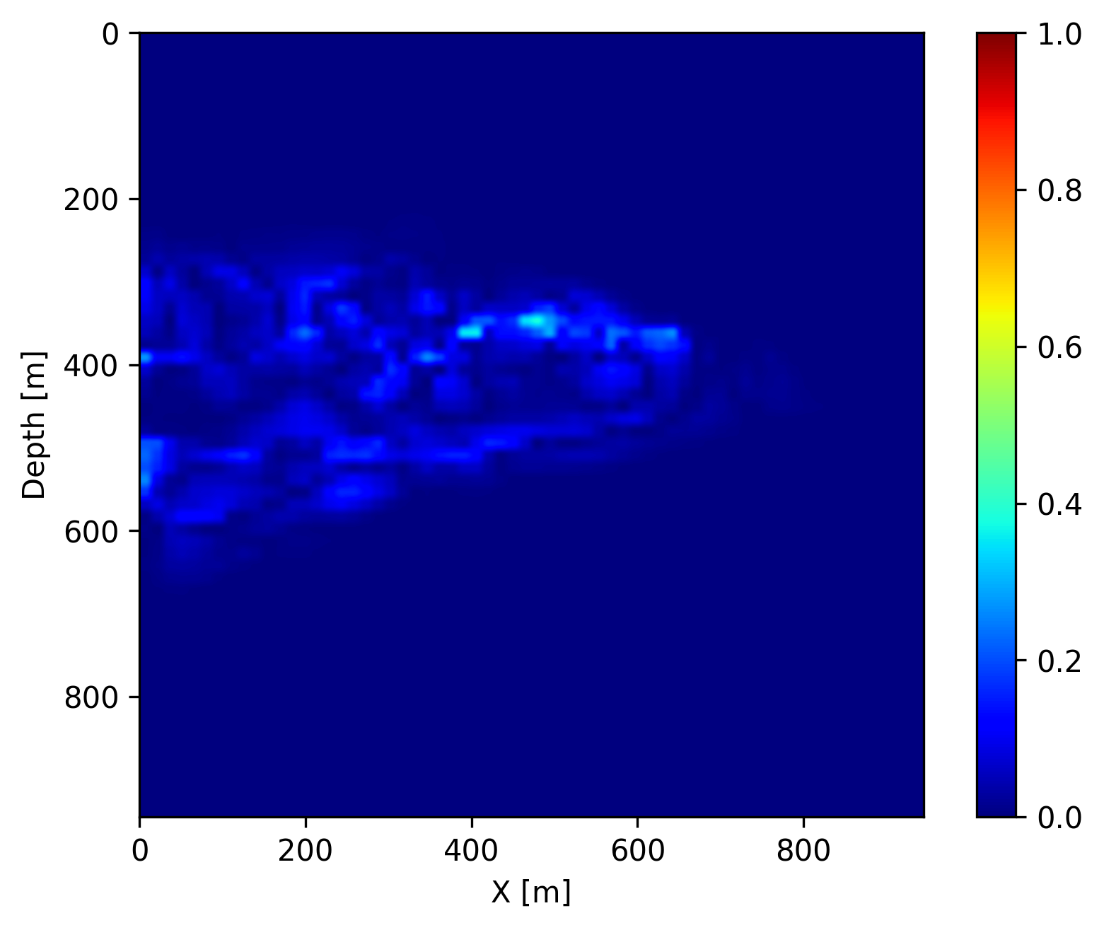
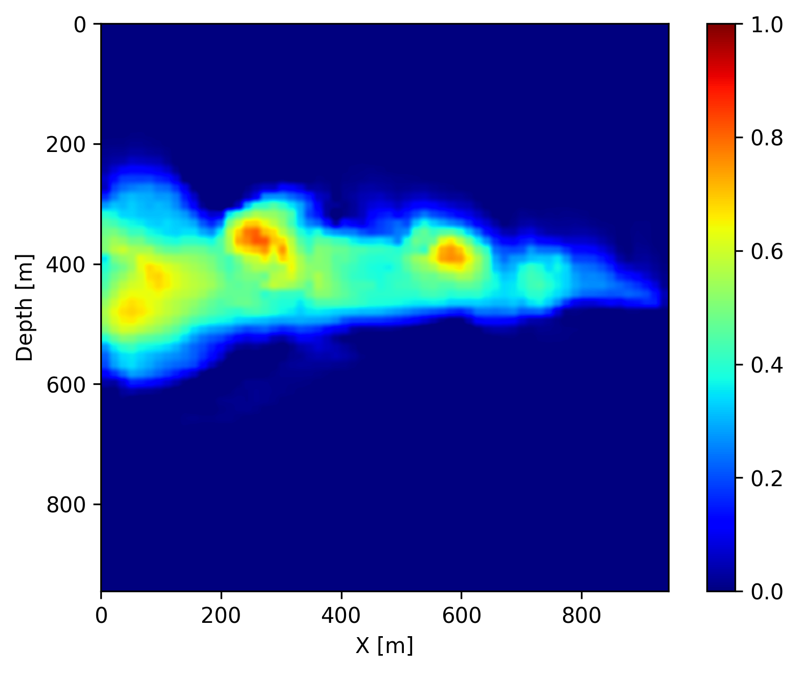
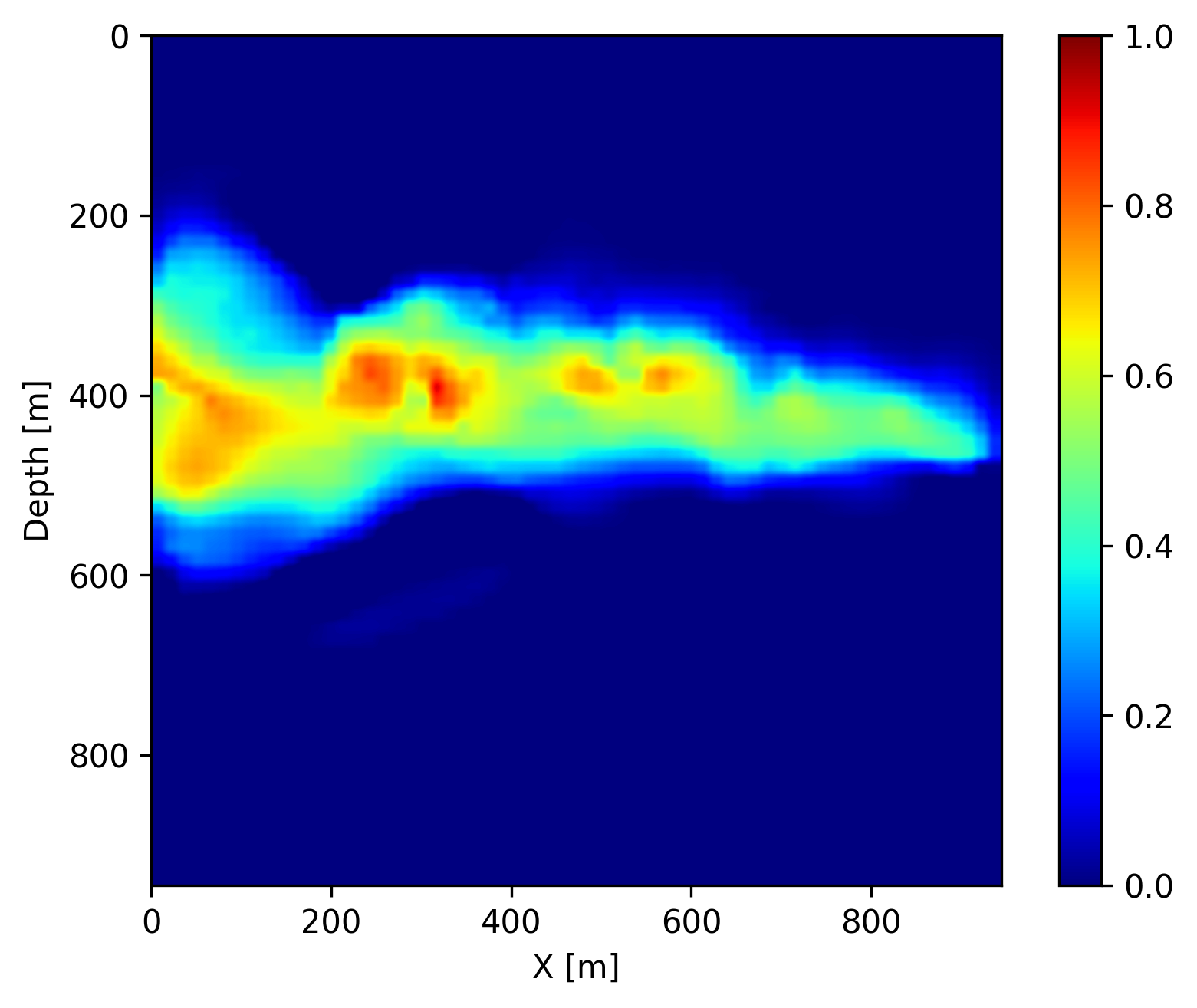
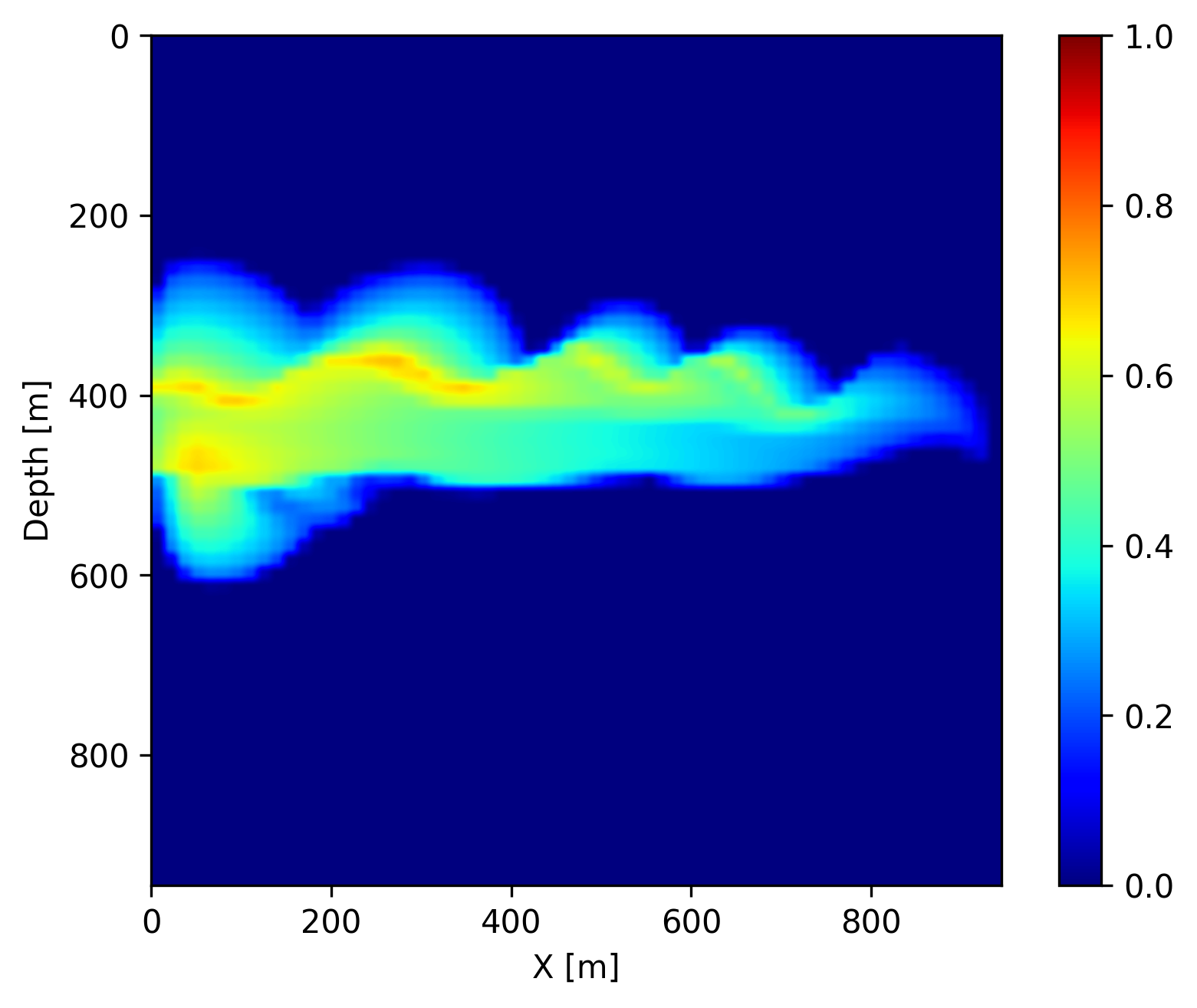
Finally, once we reach the \(400\) days, we do not have access to seismic data anymore (in the future). However, we can use the trained FNO to forecast the CO₂ concentration in the relatively near future assuming that the fluid dynamic will not drastically change. We show on Figure 4 the forecast at day \(440\), \(560\) and \(680\) by juxtaposing them with the ground truth obtained through numerical simulation and the differences. We observe that the forecast is relatively accurate and catches the global behavior of the plume even though no seismic monitoring data is available. This result confirms that the pre-trained FNO in combination with the permeability estimate from the time-lapse seismic can provide a forecasting framework for seismic monitoring of geological carbon storage.

The learned coupled inversion framework is implemented in Julia, where we use Flux.jl for AD. The scripts to reproduce the experiments are available on the SLIM GitHub page https://github.com/slimgroup/FNO4CO2.

Discussion and conclusion

Coupled inversion for carbon sequestration monitoring is computationally challenging as it needs to iteratively solve fluid-flow and wave equations, and differentiate through the solvers. We overcome this problem by replacing the fluid-flow solver by a pre-trained Fourier neural operator, which reduces the computational cost of fluid-flow simulations and differentiation. We demonstrated that the learned coupled inversion framework can yield reasonable estimates of the permeability of the reservoir. This estimated permeability can then be used for not only generating the CO₂ concentration snapshots at the current vintages, but also forecasting the growth of the CO₂ plume in the future. This can potentially enable uncertainty quantification for potential plume behaviors in the future for risk management. While these initial results on learned coupled inversion are encouraging, more realistic physics phenomena can be considered in future work to numerically model the fluid-flow and wave physics more accurately. More robust inversion methods with regularization and constraints may also lead to better estimation of the permeability and CO₂ concentration. Future work will also involve exploration of the generalization capability of the Fourier neural operator and development of a large-scale \(3\)D continuous monitoring framework that potentially updates the permeability according to the latest acquired seismic data from the field.

Acknowledgement

This research was carried out with the support of Georgia Research Alliance and partners of the ML4Seismic Center. The authors thank Philipp A. Witte at Microsoft for the constructive discussion.