Velocity continuation with Fourier neural operators for accelerated uncertainty quantification

Introduction

Seismic imaging involves estimating the short-wavelength component of the Earth’s subsurface squared-slowness model—known as the seismic image—given shot records and an estimation of the smooth background squared-slowness model. This linearized imaging problem is challenged by the computationally expensive forward operator as well as presence of measurements noise, linearization errors, modeling errors, and the nontrivial nullspace of the linearized forward Born modeling operator (Lambaré et al., 1992; Schuster, 1993; Nemeth et al., 1999). These challenges highlight the importance of uncertainty quantification (UQ) in seismic imaging, where instead of finding one seismic image estimate, a distribution of seismic images is obtained that explains the observed data (Tarantola, 2005), consequently reducing the risk of data overfit and enabling UQ (Malinverno and Parker, 2006; Martin et al., 2012; Ray et al., 2017; Zhu et al., 2016; Fang et al., 2018; G. K. Stuart et al., 2019; Herrmann et al., 2019; Siahkoohi et al., 2020a, 2020b, 2021; Siahkoohi and Herrmann, 2021).

The seismic imaging uncertainty can be attributed to two main sources (Thore et al., 2002; Osypov et al., 2013; Ely et al., 2018): (1) errors in the data, which include measurement and linearization errors; and (2) modeling errors, which include errors in the estimation of the background squared-slowness model. In this paper, we focus on uncertainties with respect to the background model as it has the main contributing factor to imaging uncertainty due to its effect on reflector positioning (Fomel and Landa, 2014; O. V. Poliannikov and Malcolm, 2016; Ely et al., 2018). To this end, we assume there are no measurement or linearization errors and consider the map from shot records to the seismic image to be represented by the deterministic reverse-time migration (RTM) algorithm. In this setup, quantifying the uncertainty in seismic imaging—due to errors in the background model—involves computing numerous RTMs with all the background model posterior samples (Zhu et al., 2016; Fang et al., 2018). Due to the high-dimensionality of seismic images, the number of seismic imaging posterior samples required to obtain accurate estimations of the imaging posterior moments is large, making UQ with respect to the background model computationally expensive for 2D and unfeasible for large 3D problems. These costs can be alleviated via velocity continuation methods (Fomel, 2003a, 2003b; Duchkov and De Hoop, 2009; Leeuwen and Herrmann, 2012; M. Yang et al., 2021) that map seismic images associated with one background model to another, without directly solving the imaging problem. Velocity continuation methods are designed to be frugal compared to computing a new RTM for each new background model, which makes them suitable for large-scale seismic imaging uncertainty quantification (Fomel and Landa, 2014; O. V. Poliannikov and Malcolm, 2016).

While several velocity continuation methods have been proposed (Fomel, 2003a, 2003b; Duchkov and De Hoop, 2009; Leeuwen and Herrmann, 2012; M. Yang et al., 2021), they typically involve solving partial differential equations (PDEs), which can be still costly in the context of seismic imaging UQ. To address this challenge, we propose a neural network surrogate for velocity continuation that is capable of mapping seismic images associated with one background model to another with negligible computational cost. Motivated by the success of Fourier neural operators (FNOs, Z. Li et al., 2021) in approximating the solution operator of PDEs (Toledo-Marín et al., 2021; Konuk and Shragge, 2021; N. Kovachki et al., 2021), we chose them as the architecture for our neural network surrogate. Due to our main interest in accelerating velocity continuation in the context of UQ, we train a survey-specific FNO that acts as a surrogate for velocity continuation for the specific survey at hand. This choice, while not offering generalizations across different survey areas in the Earth, can speed up seismic imaging UQ for the survey at hand, which involves computing seismic images associated with many background model posterior samples. We show that the FNO can be trained using \(200\) pairs of background and seismic image pairs, making the survey-specific training procedure computationally viable. To scale this method to industry size problems, transfer learning (Yosinski et al., 2014) can further reduce the upfront costs of training the FNO. After training, the FNO can be used to obtain samples from the imaging posterior almost free of cost.

In the next section, we describe seismic imaging by introducing the forward Born modeling operator, through which the seismic image relates to the background model. Next, we define velocity continuation, followed by describing our proposed FNO-based approach for accelerating seismic imaging UQ. Finally, we evaluate the performance of the trained neural operator on a realistic dataset, and we demonstrate how the imaging uncertainty affects the positioning of the reflectors in the seismic image.

Theory

We introduce a deep-network surrogate for velocity continuation in order to enable faster quantification of uncertainty—due to errors in the background velocity model—in seismic imaging. We begin with an introduction to seismic imaging and the linearized forward model associated with it.

Seismic imaging

The inverse problem that we tackle involves the process of estimating the short-wavelength component of the Earth’s unknown subsurface squared-slowness model given measurements recorded at the surface. This problem, also known as seismic imaging, can be formulated as a linear inverse problem by linearizing the nonlinear relationship between shot records and the squared-slowness model, governed by the wave-equation. In its simplest acoustic form, the linearization with respect to the slowness model—around a background squared slowness model \(\B{m}_0\)—leads to a linear inverse problem for estimating the ground truth seismic image \(\delta \B{m}^{\ast}\) with the following forward model, \[ \begin{equation} \delta \B{d}_i = \B{J}(\B{m}_0, \B{q}_i) \delta \B{m}^{\ast}. \label{linear-fwd-op} \end{equation} \] In the above expression, \(\delta \B{d}=\left\{\delta \B{d}_{i}\right\}_{i=1}^{n_s}\) are \(n_s\) linearized shot records and \(\B{J}(\B{m}_0, \B{q}_i)\) represents the linearized Born scattering operator. This operator is parameterized by the source signature \(\B{q}_{i}\) and the background squared-slowness model \(\B{m}_0\), which is typically estimated in the previous inversion steps (Zhu et al., 2016; Fang et al., 2018). In this work, we focus on potential inaccuracies in the background model, the main source of variability and uncertainty in seismic imaging (Fomel and Landa, 2014; O. V. Poliannikov and Malcolm, 2016; Ely et al., 2018). Therefore, we assume there are not measurement and linearization errors, which leads to a deterministic mapping from \(\left\{\delta \B{d}_{i}\right\}_{i=1}^{n_s}\) to \(\delta \B{m}\) for a given background model. We use RTM for this deterministic map, which involves applying the adjoint linearized Born scattering operator to the linearized shot records for all source experiments, \[ \begin{equation} \delta \B{m}_{\text{RTM}} = \sum_{i=1}^{n_s} \B{J}(\B{m}_0, \B{q}_i)^{\top} \delta\B{d}_i. \label{rtm} \end{equation} \] Since this map is deterministic, the uncertainty in the background model can be translated into uncertainty in seismic imaging by evaluating Equation \(\ref{rtm}\) for the background models sampled from the posterior distribution \(p(\B{m}_0\mid \B{d})\), where \(\B{d}\) represents the shot records with no linearization (the field data) (Zhu et al., 2016; Fang et al., 2018). Bayesian inference involving high-dimensional posterior distributions, for example seismic imaging and full-waveform inversion, requires many samples from the posterior distribution for accurate Monte Carlo approximation of high-dimensional integrals (Gelman and Rubin, 1992). As a result, the mapping in Equation \(\ref{rtm}\) must be evaluated over numerous background model samples from \(p(\B{m}_0\mid \B{d})\), which is computationally expensive due to costs of applying \(\B{J}(\B{m}_0,\B{q}_i)^{\top},\,i=1,\ldots,n_s\). To address this computational challenge, our proposed method involves a FNO-based velocity continuation approach that is capable of mapping seismic images associated with one background model to another, effectively replacing a costly demingration-migration. We describe this approach in the next section.

Velocity continuation

At its core, velocity continuation is a process which alters a seismic image based on changes in the background model (Fomel, 2003a, 2003b; Leeuwen and Herrmann, 2012; M. Yang et al., 2021). Using this technique, an initial seismic image associated with an initial background model \(\B{m}_{\text{init}}\) is altered to approximate the seismic image associated with a target background model \(\B{m}_{\text{target}}\) without computing Equation \(\ref{rtm}\). This process can be interpreted as a map (Duchkov and De Hoop, 2009): \[ \begin{equation} \mathcal{T}_{\left(\B{m}_{\text{init}}, \B{m}_{\text{target}}\right)}: \delta \mathcal{M} \to \delta \mathcal{M}, \label{velocity-continuation} \end{equation} \] where \(\delta \mathcal{M}\) denotes the space of seismic images, and the velocity continuation map is parameterized by \(\B{m}_{\text{init}}\) and \(\B{m}_{\text{target}}\). We take advantage of recent advances in deep learning to train a surrogate model for velocity continuation that approximates \(\mathcal{T}_{\left(\B{m}_{\text{init}},\B{m}_{\text{target}}\right)} = \B{J}(\B{m}_{\text{target}},\B{q}_i)^{\top}(\B{J}(\B{m}_{\text{init}}, \B{q}_i)^{\top})^{\dagger}\), which can be evaluated virtually for free instead of solving four PDEs. Through this approach, we are able to significantly accelerate velocity continuation, trading wave-equation solves for a simple neural network inference. This is of considerable importance in the context of seismic imaging UQ. Before demonstrating the benefits of our approach, we introduce FNOs in the context of velocity continuation.

Fourier neural operators for velocity continuation

In light of their success in learning mesh-free solution operators to PDEs (Toledo-Marín et al., 2021; Konuk and Shragge, 2021; N. Kovachki et al., 2021), we choose FNOs (Z. Li et al., 2021) as a surrogate model for velocity continuation—a process that can be interpreted as a double linearized PDE solve. The main components of FNOs are the Fourier layers, which involve a Fourier transform over the spatial dimensions of their input, followed by a learned pointwise multiplication and an inverse Fourier transform. These layers act as long-kernel convolutional layer, akin to pseudo-spectral methods, which explains the representation power of FNOs (N. Kovachki et al., 2021). To train a FNO as a surrogate model for velocity continuation, we define it as a map \[ \begin{equation} \mathcal{G}_{\B{w}} : \mathcal{M} \times \delta \mathcal{M} \to \delta \mathcal{M}, \label{fno-map} \end{equation} \] where \(\mathcal{G}_{\B{w}}\) denotes the FNO with weights \(\B{w}\), and \(\mathcal{M}\) is the space of background models. In words, we design \(\mathcal{G}_{\B{w}}\) as a neural network that takes as input the target background model and the initial seismic image, and outputs the target seismic image. This choice is analogous to the structure of the velocity continuation map \(\mathcal{T}_{\left(\B{m}_{\text{init}},\B{m}_{\text{target}}\right)}\) (cf. Equation \(\ref{velocity-continuation}\)), except that we fix the initial background model \(\B{m}_{\text{init}}\) to an arbitrary background model posterior sample, hence making the dependence of \(\mathcal{G}_{\B{w}}\) to \(\B{m}_{\text{init}}\) implicit. With this choice of inputs and output for \(\mathcal{G}_{\B{w}}\), the FNO’s task is to perturb the input initial seismic image according to the provided target background model in order to predict the target seismic image.

Due to our interest in accelerating velocity continuation in the context of UQ, we train a survey-specific FNO that acts as a surrogate for velocity continuation for the specific survey at hand. This choice, while not offering generalizations across different survey areas in the Earth, can speed up seismic imaging UQ for the survey at hand, which involves computing seismic images associated with many posterior background model samples \(\B{m}_0 \sim p(\B{m}_0\mid \B{d})\). By training the FNO on a small number of these background model and seismic image pairs, i.e., approximately \(200\), we can accelerate the velocity continuation process for the rest of the background model posterior samples while limiting the risk of introducing generalization errors due to the strong heterogeneity of Earth. To achieve this, we construct a set of \(N\) training input-output pairs in the form of \[ \begin{equation} \bigg\{ \Big ( \big(\B{m}_{0}^{(i)},\delta \B{m}_{\text{init}} \big),\delta \B{m}_{\text{RTM}}^{(i)} \Big) \ \Big | \ i=1,\ldots,N \bigg \}, \label{fno-training-pairs} \end{equation} \] where \((\B{m}_{0}^{(i)},\delta \B{m}_{\text{init}})\) is the input target background and initial seismic image training pair, and \(\delta \B{m}_{\text{RTM}}^{(i)}\) is the associated target seismic image. Training involves minimizing the squared \(\ell_2\)-norm of the difference between the FNO output and the target seismic image with respect to FNO weights, \[ \begin{equation} \B{w}^{\ast} = \argmin_{\B{w}}\, \frac{1}{N} \sum_{i=1} \| \mathcal{G}_{\B{w}}(\B{m}_{0}^{(i)}, \delta \B{m}_{\text{init}}) - \delta \B{m}_{\text{RTM}}^{(i)} \|_2^2. \label{fno-train} \end{equation} \] We solve optimization problem \(\ref{fno-train}\) with the Adam stochastic optimization algorithm (Kingma and Ba, 2014). After training, the trained FNO approximates the velocity continuation map for a fixed homogeneous initial background model, i.e., \[ \begin{equation} \mathcal{G}_{\B{w}^{\ast}}(\B{m}_{\text{target}}, \delta \B{m}_{\text{init}}) \approx \mathcal{T}_{\left(\B{m}_{\text{init}}, \B{m}_{\text{target}}\right)} (\delta \B{m}_{\text{init}}) = \delta \B{m}_{\text{target}}, \label{fno-approx} \end{equation} \] where \(\B{m}_{\text{init}}\) is fixed to an arbitrary background model posterior sample and \(\delta \B{m}_{\text{target}}\) denotes the seismic image associated with \(\delta \B{m}_{\text{init}}\). Given background model samples \(\B{m}_0 \sim p(\B{m}_0\mid \B{d})\) as input, the FNO outputs samples from the imaging posterior, \(p(\B{m}_0\mid \delta \B{d})\). This process accelerates seismic imaging uncertainty quantification as no further RTMs (Equation \(\ref{rtm}\)) need to be computed. Training the FNO with as little as \(200\) training pairs makes the survey-specific training procedure computationally viable. To further accelerate the process, training of the FNO can be started as the same time as the background model posterior sampling phase, using the already collected posterior samples as training data. In the next section, we show the results of approximating the velocity continuation map with a FNO via a quasi-real seismic experiment.

Numerical experiments

The purpose of the presented numerical experiments here is to demonstrate the ability to approximate the velocity continuation map (Equation \(\ref{velocity-continuation}\)) using a FNO. We further show how this trained FNO can be used for UQ by showing the effect of imaging uncertainty on the positioning of the reflectors. We begin by describing the training setup, including the seismic acquisition geometry.

Acquisition geometry and training configuration

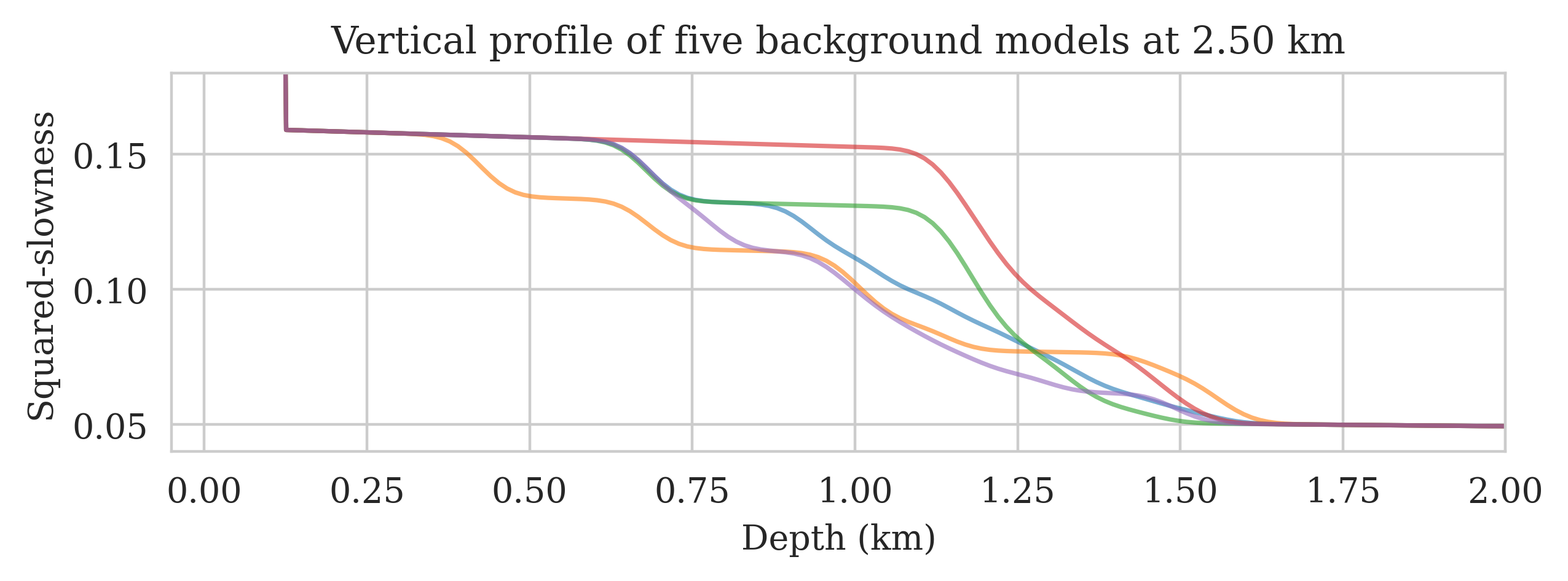
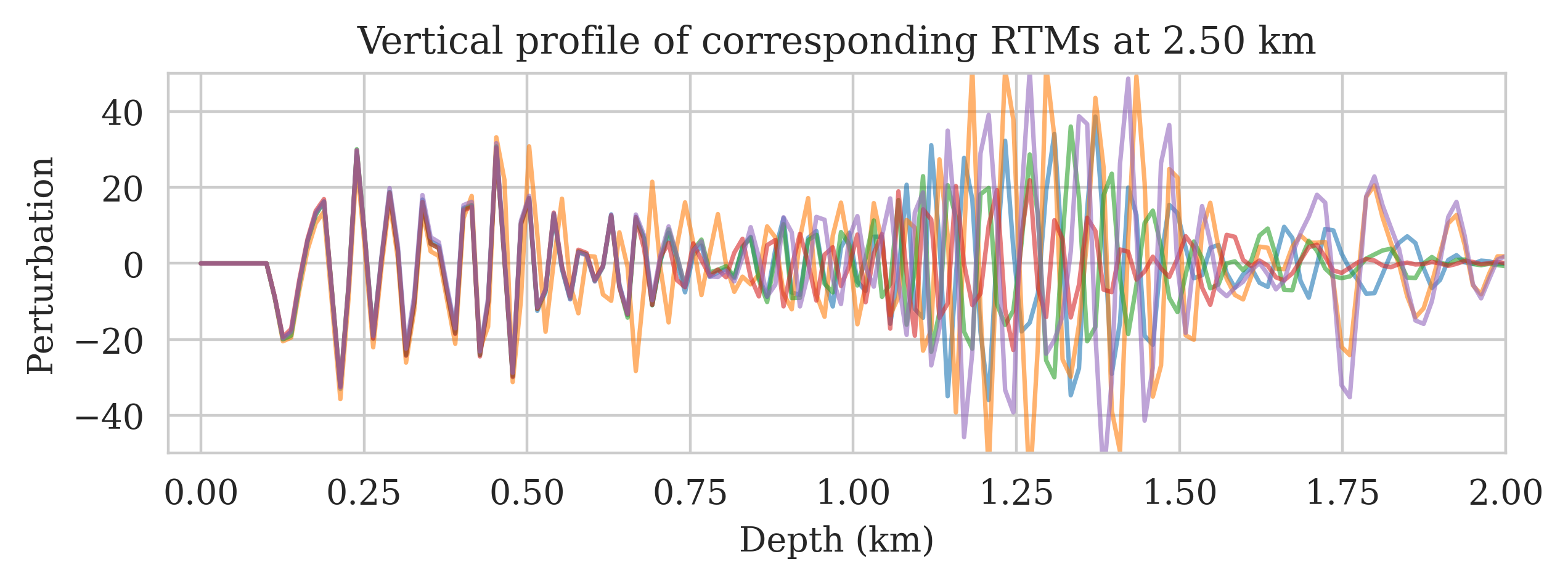
Our examples involve imaging a 2D subset of the Parihaka (Veritas, 2005; WesternGeco., 2012) prestrack Kirchhoff migration field dataset. We use this 2D section to create linearized data according to the linear forward model in Equation \(\ref{linear-fwd-op}\), where we consider no measurement and linearization errors. The model is discretized on a \(12.5\,\mathrm{m}\) vertical and \(20\,\mathrm{m}\) horizontal grid, and the data is acquired with \(102\) equally spaced sources and \(204\) fixed receivers. We use a Ricker wavelet with a central frequency of \(30\, \mathrm{Hz}\) as the source signature. For presentation purposes, we augment a \(125\, \mathrm{m}\) water column on top of these models to limit the near source imaging artifacts. We create background models by assuming access to an oracle, which provides geologically consistent background models with the 2D section. Given \(200\) background models, we migrate the simulated seismic data via Equation \(\ref{rtm}\) to obtain the corresponding seismic images. Figures 1a and 1b show the vertical profile of five randomly selected background and seismic images at \(2.50\,\mathrm{km}\), respectively. These images, displaying strong amplitude and phase differences, highlight the importance of quantifying the uncertainty in imaging when dealing with errors in the background model. To reduce the costs associated with UQ, we train the FNO surrogate using the \(200\) training pairs (cf. Equation \(\ref{fno-training-pairs}\)) for \(500\) epochs with the Adam optimizer (Kingma and Ba, 2014).

Results

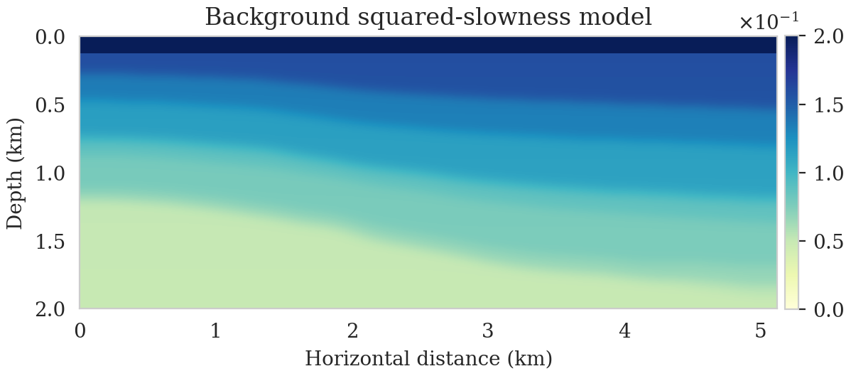
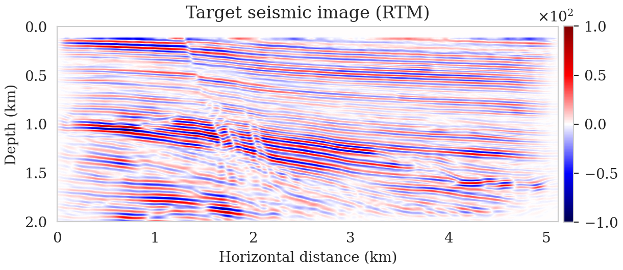
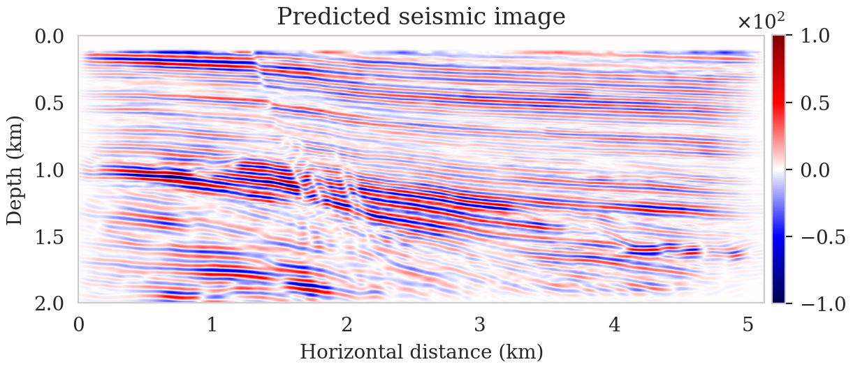
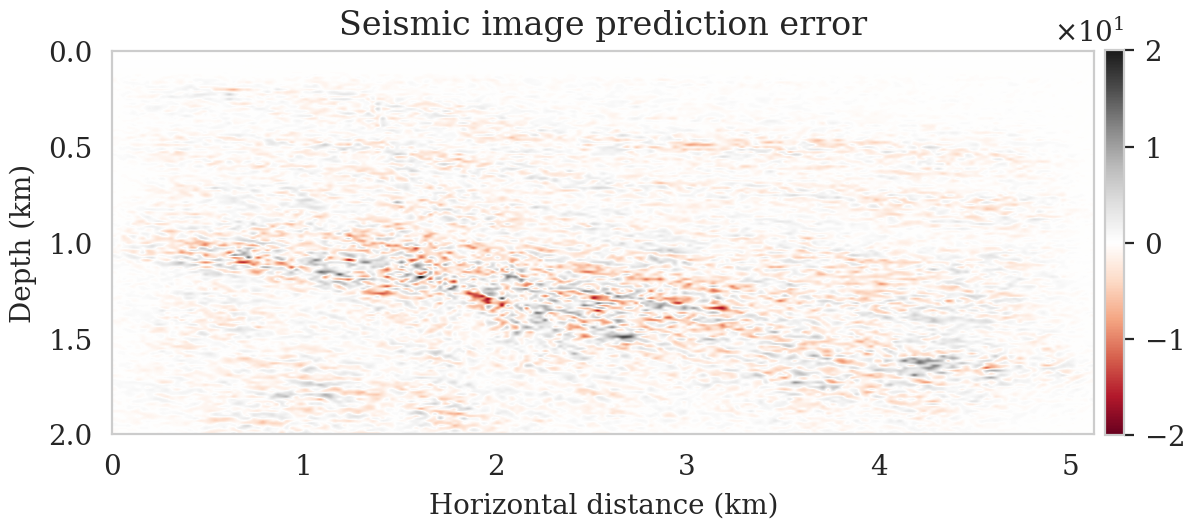
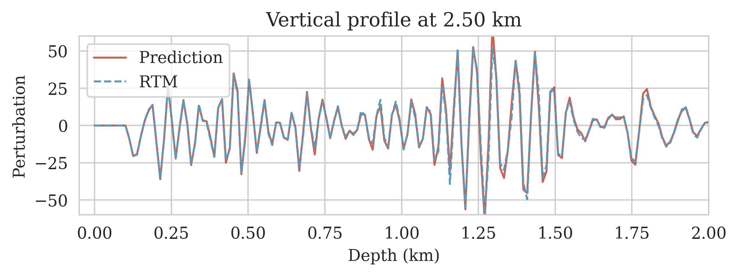
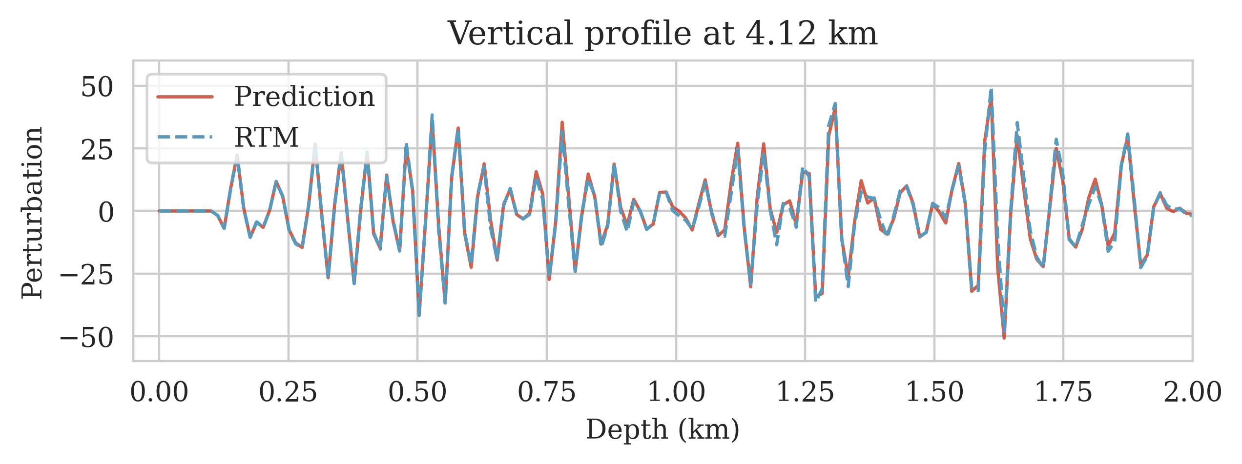
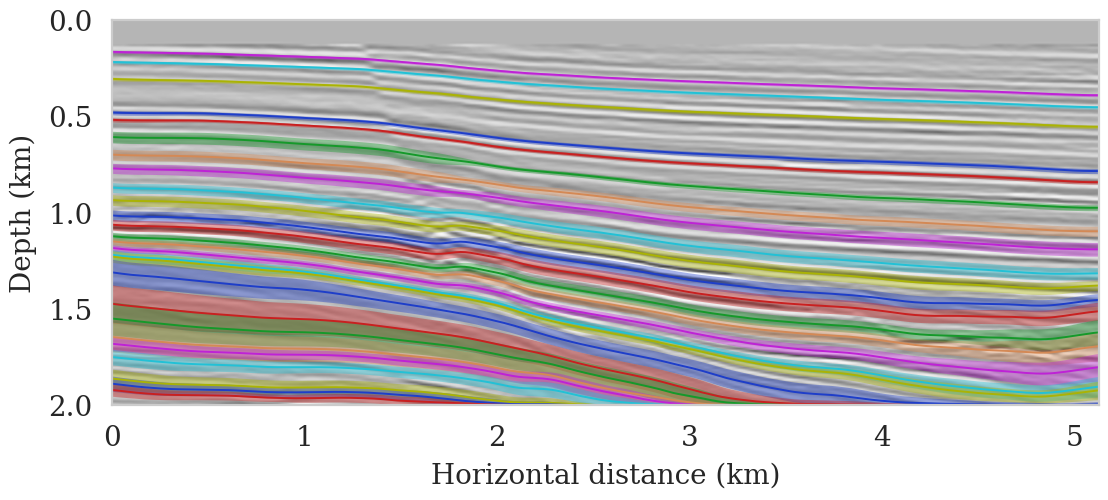
To evaluate the accuracy of the trained FNO in predicting seismic images, we compare its output to the target seismic image, i.e., the RTM image obtained via Equation \(\ref{rtm}\) when using the target background model (Figure 2a) to parameterize the Born scattering forward operator. This is conducted over the testing dataset, which is derived using the same procedure as the training dataset using the background model creating oracle. Figures 2b and 2c show the target and predicted seismic images, respectively, and Figures 2d includes the difference between them. We observe that the network has accurately predicted the target image, where errors are mostly due to amplitude differences. The accuracy of the prediction in terms of phase and amplitude can be further confirmed by focusing on two vertical profiles, at \(2.50\,\mathrm{km}\) (Figure 2e) and \(4.125\,\mathrm{km}\) (Figure 2f) horizontal locations, which include regions with fault and torturous reflectors. We use the trained FNO for UQ by providing testing background models and predicting the associated seismic images. We visualize the obtained uncertainties by showing the variability in the location of reflectors, determined via an automatic horizon tracking software (X. Wu and Fomel, 2018). We pass the seismic images predicted by the FNO to the horizon tracker for \(25\) selected horizons. As a result, we obtain multiple instances of each horizons, from which we compute pointwise mean and standard deviations. Figure 3 indicates the result where the solid lines correspond to the mean among different instances of each horizons and shaded areas indicate the mean plus and minus the pointwise standard deviation. These shaded areas indicate uncertainties in the location of the reflectors, which are due to the variability in the background models. As expected, we find a general increase of uncertainty with depth. We also observe that the areas of high uncertainty are correlated with areas of poor illumination, faults and tortuous reflectors.

In this example, we use Devito (Luporini et al., 2018; Louboutin et al., 2019) for the wave-equation based simulations. We based our PyTorch FNO implementation on the original implementation. The code to reproduce our results are made available on GitHub.

Conclusions and discussion

Quantifying the uncertainty in seismic imaging due to errors in the background model involves solving many seismic imaging problems that vary in the parameterization of the background model of the forward operator. To reduce the computational cost of this process—mainly due to the computational costs of the forward operator—we proposed to train a survey-specific Fourier neural operator surrogate that mimics velocity continuation. This surrogate model maps seismic images associated with one background model to another virtually for free, which has the benefit of accelerating uncertainty quantification. We showed that this surrogate model can be trained with as few as \(200\) training pairs while still providing a good seismic image prediction accuracy. Further research is required in training a reliable global surrogate, being able to generalize across other survey areas and more realistic physics.

Acknowledgment

This research was carried out with the support of Georgia Research Alliance and partners of the ML4Seismic Center.