A practical workflow for land seismic wavefield recovery with weighted matrix factorization

Introduction

One of the critical phases in the early stages of oil and gas exploration is seismic data acquisition. Inspired by relatively recent developments encouraged by the field of Compressive Sensing (Candès et al., 2006), seismic data is increasingly collected randomly along the spatial coordinates to shorten the acquisition time and to reduce cost. While random sampling improves acquisition productivity (Mosher et al., 2014), it does shift the burden from field acquisition to data processing (Chiu, 2019) since fully sampled seismic data is a prerequisite to subsequent steps such as multiple removal and migration.

Wavefield recovery is one of the key steps to reconstruct fully seismic data from subsampled data. Recovery methods based on wavefield reconstruction that exploits data sparsity in different transform domains, such as wavelet (Villasenor et al., 1996), Fourier (M. D. Sacchi et al., 1998), and curvelet (Herrmann and Hennenfent, 2008), have been proposed. More recently, several seismic studies have investigated wavefield recovery via low-rank matrix factorizations (Kumar et al., 2015), which are relatively simple and computationally cheap. The general idea of these methods is to exploit low-rank structure of fully sampled frequency slices when they are organized in a matrix. Oropeza and Sacchi (2011) and Kumar et al. (2015) showed that the presence of noise or missing traces increases the rank of these matrices, and they used this property to recover the fully sampled frequency slices via low-rank matrix factorization.

While the low-rank matrix factorization method has had some success, especially for low to midrange frequencies, it struggles to recover high frequency slices, which require higher ranks because they cannot be accurately approximated by low-rank factorizations. To solve this problem, A. Aravkin et al. (2014), Eftekhari et al. (2018), and Zhang et al. (2019) used the wavefield recovery via weighted matrix factorization to reconstruct seismic data by introducing matrix weights defined in terms of factorizations at neighboring frequencies that live in close-by subspaces. By moving the matrix weights from the constraint to the data-misfit term, Zhang et al. (2020) proposed a computationally more efficient scheme capable of handling high frequencies.

Even though this weighted approach has had success, there remains the challenge that land seismic data contains ground roll, which because of its strong amplitude and high spatial frequency content is known to (Liu, 1999) degrade the wavefield reconstructions based on promoting structure whether this is sparsity or low rank. The reason for this possible degradation is two-fold. First, groud roll corresponds to Rayleigh-type surface waves, which are slow and for this reason often aliased. Second, ground roll has strong amplitudes, which causes the reconstruction to focus on the ground roll at the expense of reconstructing the low-amplitude body waves. While ground roll is typically dominant at the low temporal frequencies, its separation from body waves is complicated by the fact that it is spatially aliased. By reconstructing the wavefield to a fine grid, where the ground roll is no longer aliased, we allow for a separation of ground roll and body waves using \(f-k\) filtering (Yilmaz, 2001) or Radon domain techniques (Trad et al., 2003). During this talk, we present a practical workflow aimed at removing the complications of carrying out wavefield reconstruction on land data dominated by ground roll.

We organize this expanded abstract as follows. First, we discuss the seismic wavefield reconstruction via weighted matrix factorization. Next, we discuss the impact of ground roll. And then, we introduce our proposed practical workflow step by step. We conclude by demonstrating our approach on synthetic \(3\)D data simulated from the Barrett model and show improved recovery quality compared to the conventional workflow.

Reconstruction with weighted matrix factorizations

In A. Aravkin et al. (2014), Eftekhari et al. (2018) and Zhang et al. (2019), the authors proposed a wavefield recovery via weighted matrix factorization. These factorizations are carried out on data organized in monochromatic frequency slices and involve the following optimization problem: \[ \begin{equation} \begin{aligned} & \minim_{\vector{X}_i} \quad \|\vector{Q}\vector{X}_i\vector{W}\|_*\\ & \text{subject to} \quad \|\mathcal{A}(\vector{X}_i) - \vector{B}_i\|_F \leq \eta. \end{aligned} \label{eqWlrmf} \end{equation} \] In this expression, the symbol \(\|\cdot\|_*\) represents the nuclear norm, given by the sum of the singular values, and \(\|\cdot\|_F\) denotes the Frobenius norm, the energy of the matrix entries. The matrix \(\vector{X}_i\), for \(i \in [1, \ldots , N_f]\), represents a fully sampled monochromatic frequency slice at the \(i\mathrm{th}\) frequency. \(N_f\) corresponds to the number of frequencies, and the matrix \(\mathcal{A}(\cdot)\) represents a mask operator used to subsample the fully sampled frequency slice. The matrix \(\vector{B}_i\) represents the observed input data with missing traces at the \(i\mathrm{th}\) frequency. The misfit tolerance \(\eta\) depends on the noise level in the observed data.

To exploit the fact that seismic data exhibits low-rank behavior in the so-called non-canonical organization (Kumar et al., 2015), we matricize the frequency slices in the source-x receiver-x organization—i.e., the to-be-recovered monochromatic data is represented by the matrix \(\vector{X}_i \in \mathbb{C}^{(N_{sx}\times N_{rx}) \times (N_{sy}\times N_{ry})}\) where \(N_{sx}\), \(N_{sy}\) are the number of sources along the \(x\) and \(y\) coordinates, respectively. \(N_{rx}\), \(N_{ry}\) are the corresponding numbers of receivers. The \(\{\vector{Q},\vector{W}\} \in \mathbb{C}^{(N_{sx}\times N_{rx}) \times (N_{sx}\times N_{rx})}\) are the weighting matrices, which include information on the subspaces of a neighboring factorization as we reconstruct the wavefield from low-to-high frequencies (Zhang et al., 2019). These weighting matrices are given by \[ \begin{equation} \vector{Q} = {w}_{1}\vector{U}\vector{U}^H + \vector{U}^\perp \vector{U}^{{\perp}{H}} \label{eqprojl} \end{equation} \] and \[ \begin{equation} \vector{W} = {w}_{2}\vector{V}\vector{V}^H + \vector{V}^\perp \vector{V}^{{\perp}{H}}. \label{eqprojr} \end{equation} \] In these expressions, the symbol \(^{H}\) denotes the Hermitian transpose. The projection matrices \(\vector{U} \in \mathbb{C}^{(N_{sx} \times N_{rx}) \times r}\), \(\vector{V}\in \mathbb{C}^{(N_{sy}\times N_{ry}) \times r}\) contain rank \(r\) column and row subspaces that derive from neighboring (lower) frequencies. The matrices \(\vector{U}^\perp\), \(\vector{V}^\perp\) are the orthogonal complements of \(\vector{U}\), \(\vector{V}\). Because factorizations of neighboring (lower) frequencies share information with the current frequency slice, they can serve as prior information aiding the wavefield recovery. The scalars \({w}_{1} \in \left(0,1 \right]\) and \({w}_{2} \in \left(0,1 \right]\) quantify the similarity between prior information and the current to-be-recovered frequency slice. Small values for these scalars indicate that we have more confidence in the prior information.

As shown in (Zhang et al., 2019), considerable improvements can be made during the recovery when reliable prior information is available. However, including weighting matrices in the nuclear norm objective function complicates the optimization making the minimization in equation \(\ref{eqWlrmf}\) computationally more expensive. To avoid this issue, we follow Zhang et al. (2020) and rewrite equation \(\ref{eqWlrmf}\) into \[ \begin{equation} \begin{aligned} & \minim_{\vector{\tilde {X}}_i} \quad \|\vector{\tilde {X}}_i\|_* \\ & \text{subject to} \quad \|\mathcal{A}({\vector{Q}^{-1}}\vector{\tilde{X}}_i{\vector{W}^{-1}}) - \vector{B}_i\|_F \leq \eta . \end{aligned} \label{eqWlrmfv2} \end{equation} \] To arrive at this formulation, we replace the optimization variable with \(\vector{\tilde{X}}_{i} = \vector{Q}\vector{X}_i\vector{W}\). After solving equation \(\ref{eqWlrmfv2}\), the original solution \(\vector{X}_i\) can be recovered by \(\vector{X}_i=\vector{Q}^{-1}\vector{\tilde{X}}_i\vector{W}^{-1}\). Mathematically, equations \(\ref{eqWlrmf}\) and equation \(\ref{eqWlrmfv2}\) are equivalent except that the solution of the second formulation is easier to compute by moving the weighting matrices to the data misfit constraint.

To prevent computationally expensive singular value decompositions (SVDs) part of the nuclear norm computations, we write equation \(\ref{eqWlrmfv2}\) in the following factored form: \[ \begin{equation} \begin{aligned} & \minim_{\vector{\tilde L}_i, \vector{\tilde R}_i} \quad \frac{1}{2} {\left\| \begin{bmatrix} \vector{\tilde L}_i \\ \vector{\tilde R}_i \end{bmatrix} \right\|}_F^2 \\ & \text{subject to} \quad \|\mathcal{A}{({\vector{Q}^{-1}} \vector{\tilde L}_i \vector{\tilde R}_i^{H} {\vector{W}^{-1}})} - \vector{B}_i\|_{F} \leq \eta. \end{aligned} \label{eqwlrf} \end{equation} \] In this expression, the \(\vector{\tilde L}_i \in \mathbb{C}^{(N_{sx}\times N_{rx}) \times r}\) and \(\vector{\tilde R}_i \in \mathbb{C}^{(N_{sy}\times N_{ry}) \times r}\) represent the low-rank factorization of \(\vector{\tilde X}_i\) with rank \(r \ll \min(N_{sx}\times N_{rx}, N_{sy}\times N_{ry})\) (Zhang et al., 2020).

While wavefield recovery based on weighted matrix factorization has been applied successfully (see e.g., Zhang et al. (2019) and Zhang et al. (2020)), its performance is challenged by data that contains strong-amplitude aliased ground roll. Because of its large-amplitude, ground roll dominates the reconstruction at the expense of body waves that are of prime interest. In the next section, we will introduce a practical workflow addressing this challenge.

Impact of ground roll

Acquisition and processing of land data are often challenged because it is contaminated by strong ground roll. Because ground roll is slow, it is often spatially aliased, complicating subsequent processing efforts to remove this coherent noise component with \(f-k\) or Radon filtering (Yilmaz, 2001, Trad et al. (2003)). Unfortunately, it is financially unfeasible to decrease the periodic receiver sampling interval to avoid aliasing (Bahia et al., 2020), and we have to resort to alternative randomized acquisition methodologies (Mosher et al., 2014, Kumar et al. (2015)) that are in principle conducive to in silico unaliased wavefield reconstruction. While this has proven to work, the presence of strong-amplitude ground roll complicates wavefield reconstruction.

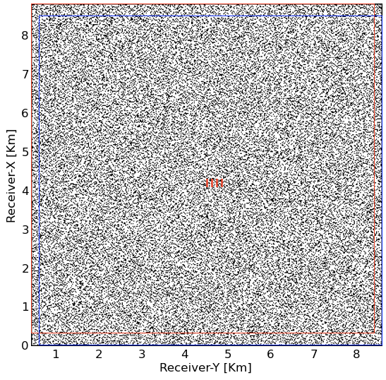
To investigate this issue, we collaborate with Klaas Koster from Occidental to conduct a blind study where we were provided with a subset consisting of \(21\) source lines, extracted from the synthetic \(3\)D SEAM Barrett dataset (Van De Coevering et al., 2019, Tan et al. (2019)). This dataset is designed to benchmark land data processing. As part of this blind study, with the acquisition geometry plotted in Figure 1, we receive 3D shot records that are randomly subsampled along the receivers. The \(8\times 8\)km receiver aperture is moving with the source location, which means that between neighboring shots randomly sampled receivers are mostly shared while some drop-off and others are added (cf. red and blue rectangle in Figure 1). Approximately 75 percent of receiver positions are missing from the regular densely sampled periodic grid of \(12.5\)m, yielding an effective average sample interval of \(50\)m, which is well below Nyquist. The data consists of \(667\) time samples with a sample interval of \(0.006\, \mathrm{s}\). The shots are sampled periodically with a sample interval of \(25\)m in the shot-line direction and \(100\)m in the perpendicular direction.

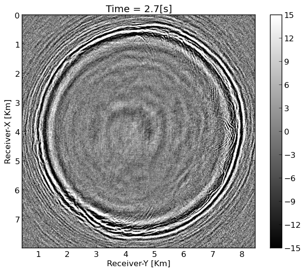
To illustrate, the effects of the strong ground roll on our factorized low-rank wavefield reconstruction scheme, we recover a patch of \(4\times 4\) shots with on the dense periodic receiver grid of \(641\) receivers in each direction sampled at \(12.5\)m. This recovery corresponds to solving a total of \(384\) monochromatic matrix factorization problems involving data volumes of \(667 \times 641 \times 641 \times 4 \times 4\). These volumes are factored into the product of two \((641\times 4)\times 340\) matrices where \(340\) is the rank \(r\). After reconstruction, the results of which are plotted in Figure 2 for a single shot record, we recover shot gathers sampled at \(12.5\)m from receivers collected at random at an average receiver spacing of \(50\)m. While we are able to recover this shot record, strong noisy artifacts remain especially at the long offsets. In addition, important reflection and diffraction information is missing and the ground roll is not well recovered making this wavefield recovery unsuitable for subsequent processing.

Proposed practical workflow

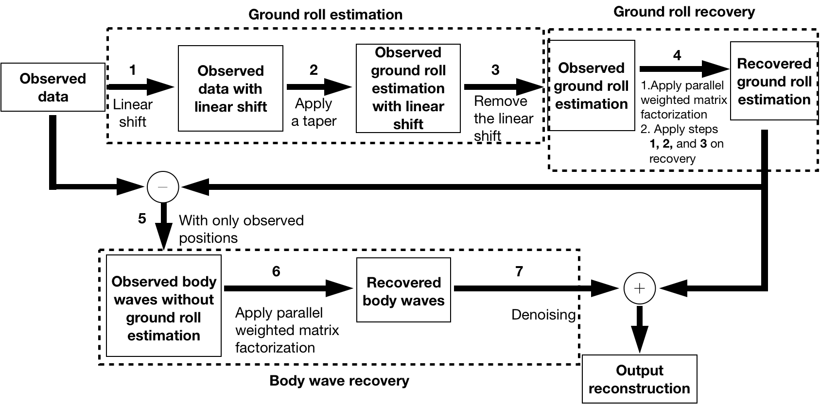
To mitigate the effects of ground roll, we propose the reconstruction of the body and surface (ground roll) waves separately. In this approach, outlined in Figure 3, we use the fact that ground roll is slow and relatively easily separable by applying a linear shift to the data. Below, we describe the different steps outlined in the dashed boxes in Figure 3.

Ground roll estimation

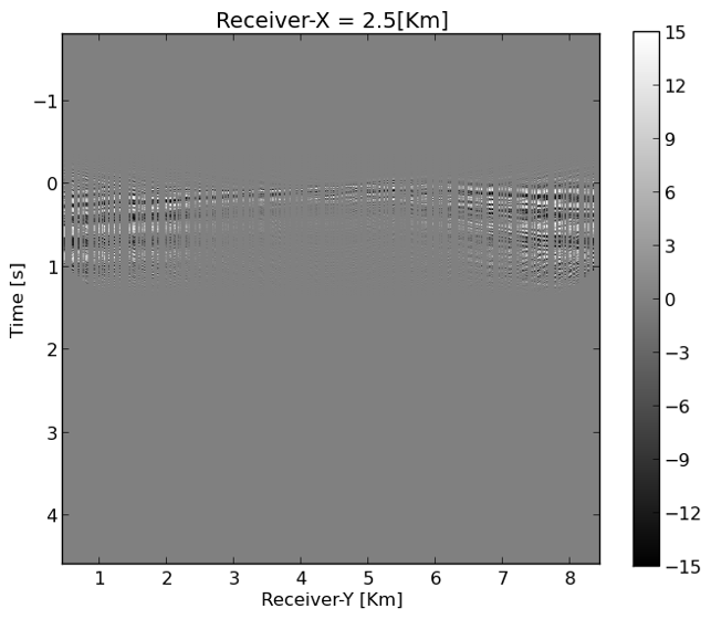
Because the ground roll is slow, it is steep and therefore at least in an approximate sense, separable from the body waves. This allows us to devise a separate reconstruction scheme to recover the ground roll before adding it back to the reconstruction of the body waves. We obtain an estimate of the ground roll by carrying out the following steps: (1) after zero-padding the input data (Figure 4a), we apply a linear shift aligning the ground roll (Figure 4b); (2) we apply a smooth taper with smooth cutoffs around at \(t=0\)s and \(t=1\)s designed to extract the ground roll (Figure 4c), followed by (3) undoing the linear shift, yielding an estimate of the randomly subsampled ground roll plotted in Figure 4d. This estimate for the ground roll serves as input for the reconstruction.

Ground roll recovery

We use the estimated ground roll as input to our wavefield reconstruction based on weighted matrix factorizations for a rank \(r=250\), which we find empirically by observing continuity of signals and limited noise in the reconstructed data. We run the reconstruction over all shots simultaneously for \(320\) iterations of SPG-\(\ell_2\) (Lopez et al., 2015) per frequency slice. To avoid reconstruction leakage, we apply steps (1)-(3) from the previous section again to get the final ground roll recovery.

Body wave recovery

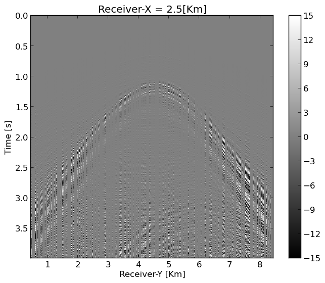
After reconstruction of the ground roll, we apply the mask \(\mathcal {A}\) to restrict the ground roll reconstruction to the observed receiver positions again and subtract it from the original subsampled input data. The resulting “ground roll free” estimate for the body waves subsequently serves as input to a second wavefield reconstruction now for the body waves. Since these waves are more complex than ground roll, we choose the rank higher (\(r=340\)). As we can observe from Figure 5, the reconstructed body waves contain, as expected, some remaining low-amplitude ground roll. Before inverse Fourier transforming the reconstructed body waves, we apply a \(f-k\) filter to each shot along both receiver coordinates to remove remnant noise. The resulting recovery for the body waves shown in Figure 5b shows reconstruction of high frequency reflected and diffracted energy. To arrive at the final result, we combine the wavefield reconstructions for the ground roll and body waves. The result of this blind study for a single shot is included in Figure 6.

Quality control (QC)

By comparing Figure 6b with Figure 2b, we observe that the proposed method produces results with less artifacts at the long offsets, and the ground roll is well recovered, especially at the near offsets (see Figure 6b for the receiver coordinate \(y\) between \(4-6\) km for the time interval \(1-1.5\) s).

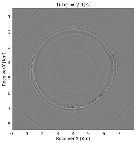
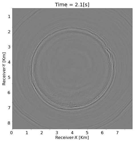
To further verify our proposed practical workflow, we sent one reconstructed shot gather to Occidental and obtained the following plots in return. Figure 7 contains time slices at \(2.1\)s with the ground truth (Figure 7a), reconstructed wavefield (Figure 7b) and difference plot (Figure 7c). From these plots, we observe that the proposed method successfully recovers body waves (reflections and diffractions) despite the presence of strong aliased ground roll. During our presentation, we will further QC our results by working with Occidental to produce stacks.

Conclusions

We presented a practical workflow successfully recovering a subset of the synthetic \(3\)D SEAM Barrett dataset randomly sampled at \(25\) percent receiver sampling. Our workflow consists of the combination of a weighted matrix factorization scheme and a separation of the subsampled input data into ground roll and body wave components. Thanks to this decomposition, we were able to mitigate the effects induced by the strong aliased ground roll. Initial findings of the blind test we carried out in collaboration with Occidental show that our method is capable of dealing with ground roll while recovering high-frequency body waves.

Related materials

The Julia code for this work is available on the SLIM GitHub page https://github.com/slimgroup/Software.SEG2021.

Acknowledgement

This research was carried out with the support of Georgia Research Alliance and partners of the ML4Seismic Center. We would like to acknowledge the support from Occidental for providing the dataset, and Georgia Institute of Technology for funding this research. We also would like to thank Klaas Koster for assisting us to carry out the blind test.