Compressive time-lapse seismic monitoring of carbon storage and sequestration with the joint recovery model

Ziyi Yin¹, Mathias Louboutin², Felix J. Herrmann^1,2
1 School of Computational Science and Engineering, Georgia Institute of Technology
² School of Earth and Atmospheric Sciences, Georgia Institute of Technology

Summary

Time-lapse seismic monitoring of carbon storage and sequestration is often challenging because the time-lapse signature of the growth of CO2 plumes is weak in amplitude and therefore difficult to detect seismically. This situation is compounded by the fact that the surveys are often coarsely sampled and not replicated to reduce costs. As a result, images obtained for different vintages (baseline and monitor surveys) often contain artifacts that may be attributed wrongly to time-lapse changes. To address these issues, we propose to invert the baseline and monitor surveys jointly. By using the joint recovery model, we exploit information shared between multiple time-lapse surveys. Contrary to other time-lapse methods, our approach does not rely on replicating the surveys to detect time-lapse changes. To illustrate this advantage, we present a numerical sensitivity study where CO2 is injected in a realistic synthetic model. This model is representative of the geology in the southeast of the North Sea, an area currently considered for carbon sequestration. Our example demonstrates that the joint recovery model improves the quality of time-lapse images allowing us to monitor the CO2 plume seismically.

Introduction

Time-lapse seismic imaging technology has recently been deployed by Carbon Capture and Storage (CCS) practitioners to monitor CO2 dynamics in porous media over long periods of time, with the Sleipner project in Norway as a pioneer (Arts et al., 2003; Furre et al., 2017). There have been several major developments to adapt compressive sensing (Janiszewski et al., 2014; F. J. Herrmann and Hennenfent, 2008) and machine learning (Bharadwaj et al., 2020; Kaur et al., 2020) to improve the productivity of (time-lapse) seismic data acquisition (Oghenekohwo et al., 2017; Wason et al., 2017) and imaging (Oghenekohwo and Herrmann, 2015) by exploiting similarities between baseline and monitor surveys. Recent work by D. Li et al. (2020) indicates the potential benefits of a coupled-physics framework where the slow-time subsurface CO2 flow, a rock physics model, and the fast-time wave physics are combined to better understand the dynamics of CO2 plumes and their effect on time-lapse seismic data for the duration of a CCS project. Because the time-lapse signal of CO2 plumes is weak, it continues to pose challenges on the robustness of time-lapse imaging (Lumley et al., 1997).

To address some of these challenges, Oghenekohwo et al. (2017);Wason et al. (2017) proposed the joint recovery model (JRM) designed to reap the benefits of low-cost randomized non-replicated acquisition. It takes advantage of the fact that time-lapse seismic data and subsurface structure undergoing localized changes share information among the different vintages. In this extended abstract, we present a synthetic case study to make the case that the dynamics of CO2 plumes can indeed be monitored with active-source surface seismic. The presented work can be considered as a continuation of recent contributions by D. Li et al. (2020), who considered seismic monitoring in a much simpler geological setting involving cross-well tomography. In our study, we consider a 2D subsection of the BG Compass model with a geology representative of the southeast of the North Sea. Blunt sandstones in this area are considered as possible reservoirs for injection of CO2. Aside from assessing the sensitivity of seismic imaging towards monitoring CO2 plumes, we also study the effects of changes in the acquisition and the presence of noise, and how the JRM can be deployed to mitigate these effects of incomplete and non-replicated data.

Our contributions are organized as follows. First, we briefly discuss full-waveform inversion and its linearization as part of time-lapse seismic imaging. Next, we introduce our joint inversion framework that explores commonalities between seismic images associated with the different vintages collected for the duration of a CCS project. We conclude by discussing a realistic time-lapse imaging experiment juxtaposing images obtained by inverting the vintages independently or jointly with JRM.

Methodology

We first briefly introduce the theoretical framework on which our wave-equation based monitoring framework for CCS is based. While we understand that more complex wave physics, e.g. elastic (Thomsen, 1986) and nonlinear inversions (Xiang Li et al., 2012), may eventually be needed, we begin by deriving a model based on the scalar wave equation parameterized by the squared slowness. We start by introducing the objective for full-waveform inversion and its linearization with respect to an assumed given smooth background model. Based on this linearization, we propose a joint recovery model, which we solve computationally efficiently with linearized Bregman iterations (Yin et al., 2008; Witte et al., 2019b).

Full-waveform inversion (FWI) and its linearization

To derive a joint wave-based seismic monitoring system, we start by introducing the objective of full-waveform inversion for the baseline (\(j=1\)) and multiple monitor surveys (\(2 \leq j \leq n_v\)) with \(n_v\geq 2\) as the number of vintages. For each vintage, this data misfit objective reads \[ \begin{equation} \underset{\mathbf{m}_j}{\operatorname{min}}\quad \|\mathbf{d}_j-\mathcal{F}_j(\mathbf{m}_j)\|_2^2 \quad \text{for}\quad j=\{1,2,\cdots,n_v\}. \label{eqfwi} \end{equation} \] In this expression, \(\mathcal{F}_j\) is the nonlinear forward modeling operator, which for given sources generates synthetic data at the receiver locations from the discretized time-lapse model parameters \(\mathbf{m}_j\). The observed data is, for each vintage, collected in the vector \(\mathbf{d}_j\). When provided with background velocity models \(\mathbf{\overline{m}}_j\) for each vintage, the above forward model can be linearized yielding \[ \begin{equation} \underset{\mathbf{\delta m}_j}{\operatorname{min}} \quad \|\mathbf{\delta d}_j-\nabla \mathcal{F}_j(\mathbf{\overline{m}}_j)\mathbf{\delta m}_j\|_2^2, \label{eqgaussnewton} \end{equation} \] where \(\mathbf{\delta d}_j=\mathbf{d}_j-\mathcal{F}_j(\mathbf{\overline{m}}_j)\) are the linearized datasets for each vintage and \(\nabla \mathcal{F}_j\) the linearized forward operator relating perturbations in the squared slowness for each vintage, \(\mathbf{\delta m}_j\), to linearized data \(\mathbf{\delta d}_j\).

Time-lapse monitoring with the joint recovery model

There exists an extensive literature on wave-based time-lapse imaging aimed at producing images that show time-lapse differences in the image space by carrying out inversion rather than imaging (Qu and Verschuur, 2017; D. Yang et al., 2016; Queißer and Singh, 2013; Maharramov et al., 2019). A prominent example of such inversion method is formed by time-lapse monitoring via double differences (Zhang and Huang, 2013; D. Yang et al., 2015) where differences are obtained by inverting differences between the monitor and baseline residuals rather than between observed and synthetic monitoring data. While this type of approach can lead to good results, it assumes the baseline and monitor surveys to be relatively noise free, well sampled, and above all replicated—i.e. the acquisition geometries between different surveys need to be identical.

In our approach, we build on a low-cost formulation for time-lapse seismic monitoring designed to handle low-cost non-replicated sparsely sampled surveys. The basic idea of this approach is to focus on what is shared amongst the different vintages rather than focusing on what is different. We argue that time-lapse monitoring benefits from such an approach if the Earth model being monitored undergoes relatively localized changes, an assumption that likely holds during CCS. To arrive at a successful joint inversion scheme, we augment the block diagonal linear system undergirding independent imaging (by minimizing Equation \(\ref{eqgaussnewton}\) independently for each vintage) with an extra column and a corresponding unknown common component. With these steps, we write \[ \begin{equation} \begin{aligned} \mathbf{A} = \begin{bmatrix} \frac{1}{\gamma}\nabla\mathcal{F}_1(\mathbf{\overline{m}}_1) & \nabla\mathcal{F}_1(\mathbf{\overline{m}}_1) & \mathbf{0} &\mathbf{0} \\ \cdots & \mathbf{0} & \cdots & \mathbf{0} \\ \frac{1}{\gamma}\nabla\mathcal{F}_{n_v}(\mathbf{\overline{m}}_{n_v}) & \mathbf{0} & \mathbf{0} & \nabla\mathcal{F}_{n_v}(\mathbf{\overline{m}}_{n_v}) \end{bmatrix}. \end{aligned} \label{eqjrm} \end{equation} \] This matrix \(\mathbf{A}\) relates the linearized data for each vintage \(\{\mathbf{\delta d}_j\}_{j=1}^{n_v}\), collected in the vector \(\mathbf{b} = \left[\mathbf{\delta d}_1^\top, \cdots, \mathbf{\delta d}_{n_v}^\top\right]^\top\), to the common component \(\mathbf{z}_0\) and innovations with respect to this common component \(\{\mathbf{z}_j\}_{i=1}^{n_v}\) all collected in the vector \(\mathbf{z} = \left[\mathbf{z}_0^\top,\cdots,\mathbf{z}_{n_v}^\top\right]^\top\). This formulation emphasizes what is common amongst the vintages when \(\gamma\) is close to \(0\), given that \(0<\gamma<n_v\) is generally a good choice in practice (Xiaowei Li, 2015).

In JRM, surveys for all vintages are explicitly related to the common component. Therefore, when acquisition geometries for different surveys are not replicated, this joint formulation recovers the common component better because the different surveys collect complementary information through the different acquisitions. As a result of the improved recovery of the common component, we can also expect the images for the different vintages themselves to be better recovered. This behavior has indeed been confirmed by several numerical experiments (Oghenekohwo and Herrmann, 2017, 2015; Wason et al., 2015) and in the presence of noise as reported by Chevron (Wei et al., 2018; Tian et al., 2018).

Time-lapse monitoring with linearized Bregman

The above joint recovery model reaps the benefit of randomized seismic acquisition with techniques adapted from Compressive Sensing, where subsampling related interferences (e.g. aliases or simultaneous source cross talk) are rendered into incoherent noise (F. J. Herrmann and Hennenfent, 2008; F. J. Herrmann, 2010). As shown by M. Yang et al. (2020);Witte et al. (2019b), these incoherent artifacts can be mapped back to coherent energy by solving the following minimization problem: \[ \begin{equation} \begin{split} \underset{\mathbf{x}}{\operatorname{min}} \quad \lambda \|\mathbf{C}\mathbf{x}\|_1+\frac{1}{2}\|\mathbf{C}\mathbf{x}\|_2^2 \\ \text{subject to}\quad \|\mathbf{b}- \mathbf{A}\mathbf{x}\|_2^2 \leq \sigma \end{split} \label{elastic} \end{equation} \] with \(\mathbf{C}\) the forward curvelet transform, \(\lambda\) a threshold parameter, and \(\sigma\) the magnitude of the noise. The advantage of this strictly convex formulation is that it can be solved via linearized Bregman iterations that for \(\sigma=0\) correspond to doing iterative soft thresholding on the dual variable—i.e., we carry out the following update at iteration \(k\) \[ \begin{equation} \begin{aligned} \begin{array}{lcl} \mathbf{u}_{k+1} & = & \mathbf{u}_k-t_k \mathbf{A}_k^\top(\mathbf{A}_k\mathbf{x}_{k}-\mathbf{b}_k)\\ \mathbf{x}_{k+1} & = & \mathbf{C}^\top S_{\lambda}(\mathbf{C}\mathbf{u}_{k+1}), \end{array} \end{aligned} \label{LBk} \end{equation} \] where \(\mathbf{A}_k\) represents the matrix in Equation \(\ref{eqjrm}\) for a subset of shots randomly selected from sources in each vintage. The vector \(\mathbf{b}_k\) contains the extracted shot records from \(\mathbf{b}\) and the symbol \(^\top\) refers to the adjoint. Sparsity is promoted via curvelet-domain soft thresholding \(S_{\lambda}(\cdot)=\max(|\cdot|-\lambda,0)\operatorname{sign}(\cdot)\) with \(\lambda\) as the threshold.

Compared to other \(\ell_1\)-norm solvers, linearized Bregman iterations are relatively simple to implement and have shown to work well in the context of least-squares imaging (M. Yang et al., 2020; Witte et al., 2019b) as long as the steplength \(t_k\) and threshold \(\lambda\) are appropriately chosen. A general choice of dynamic steplength \(t_k\) is given by \(t_k=\|\mathbf{A}_k\mathbf{x}_k-\mathbf{b}_k\|_2^2 / \|\mathbf{A}_k^\top(\mathbf{A}_k\mathbf{x}_k-\mathbf{b}_k)\|_2^2\)(Lorenz et al., 2014) and the threshold \(\lambda\) is typically chosen to be proportional to the maximum of \(|\mathbf{u}_k|\) in the first iteration (\(k=1\)). After solving problem \(\ref{elastic}\) by the iterative process \(\ref{LBk}\), estimates for the baseline and monitor images are obtained via \(\widehat{\mathbf{\delta m}}_j=\widehat{\mathbf{x}}_0+\widehat{\mathbf{x}}_j,\, j=1,2,\cdots,n_v\) where \(\widehat{\mathbf{x}}\) minimizes problem \(\ref{elastic}\).

Numerical Case Study Blunt Sandstone SW North Sea

By means of a realistic synthetic experiment, we demonstrate deployment of the joint recovery model to monitor CCS. To create a realistic monitoring scenario, we start by modeling the development of a CO2 plume with a numerical scheme that solves the two-phase flow equation. Next, we translate the CO2 concentration to time-lapse changes in acoustic wavespeed perturbations, which we use to generate seismic data for the vintages. These datasets, collected with different acquisitions, serve as input to our imaging scheme.

Geologic and rock physical setting

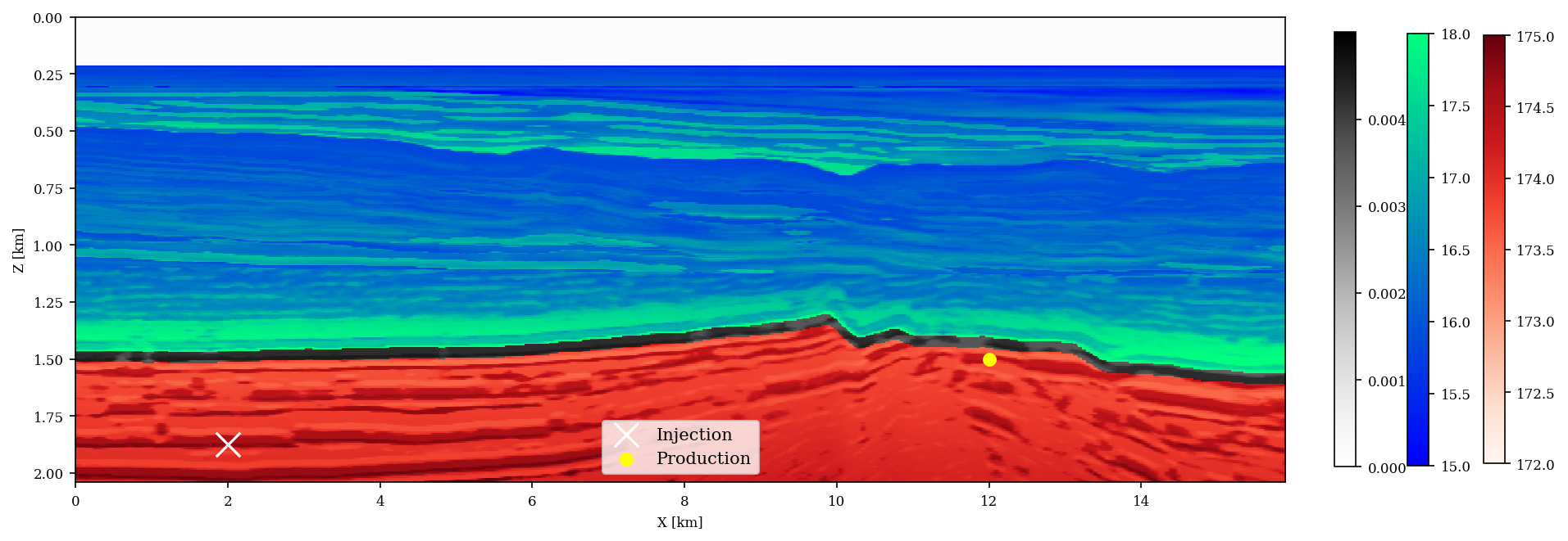
To numerically validate the potential improvement of time-lapse monitoring via our joint recovery model, we consider the 2D \(2\times 15.9\)km subset of the BG Compass model plotted in Figure 1. This figure contains a plot of the spatial distribution for the permeability and is representative for CCS in Blunt sandstones. Following the stratigraphy in the real setting, the synthetic stratigraphic section in Figure 1 can roughly be divided into three main sections, namely (i) the highly porous (average \(22\%\)) and permeable (\(> 170\)mD) Bunter Sandstone of about \(300-500\)m thick and that serves as the CO2 reservoir (red area in Figure 1, which includes location of the injection well, denoted by the white \(\times\), and the production well denoted by the yellow \(\bullet\)); (ii) the primary seal (permeability \(10^{-4}-10^{-2}\)mD) made of the Rot Halite Member, which is \(50\)m thick and is typically continuous (black layer in Figure 1); (iii) the secondary seal made of the Haisborough group, which is \(>300\)m thick and consists of low-permeable (permeability \(15-18\)mD) mudstones.

By assuming a linear relationship between the compressional wavespeed and permeability in each stratigraphic section, we arrive at the synthetic permeability model plotted in Figure 1. To convert wavespeed to permeability, we assume for each section that an increase of \(1\)km/s in the compressional wavespeed corresponds to an increase of \(1.63\)mD in the permeability. Given these values for the permeability, we derive values for the porosity using the Kozeny-Carman equation (Costa, 2006) \(K = \mathbf{\phi}^3 \left(\frac{1.527}{0.0314*(1-\mathbf{\phi})}\right)^2\), where \(K\) and \(\phi\) denote permeability (mD) and porosity (%) with constants taken from the Strategic UK CCS Storage Appraisal Project report.

Simulation of CO2 dynamics

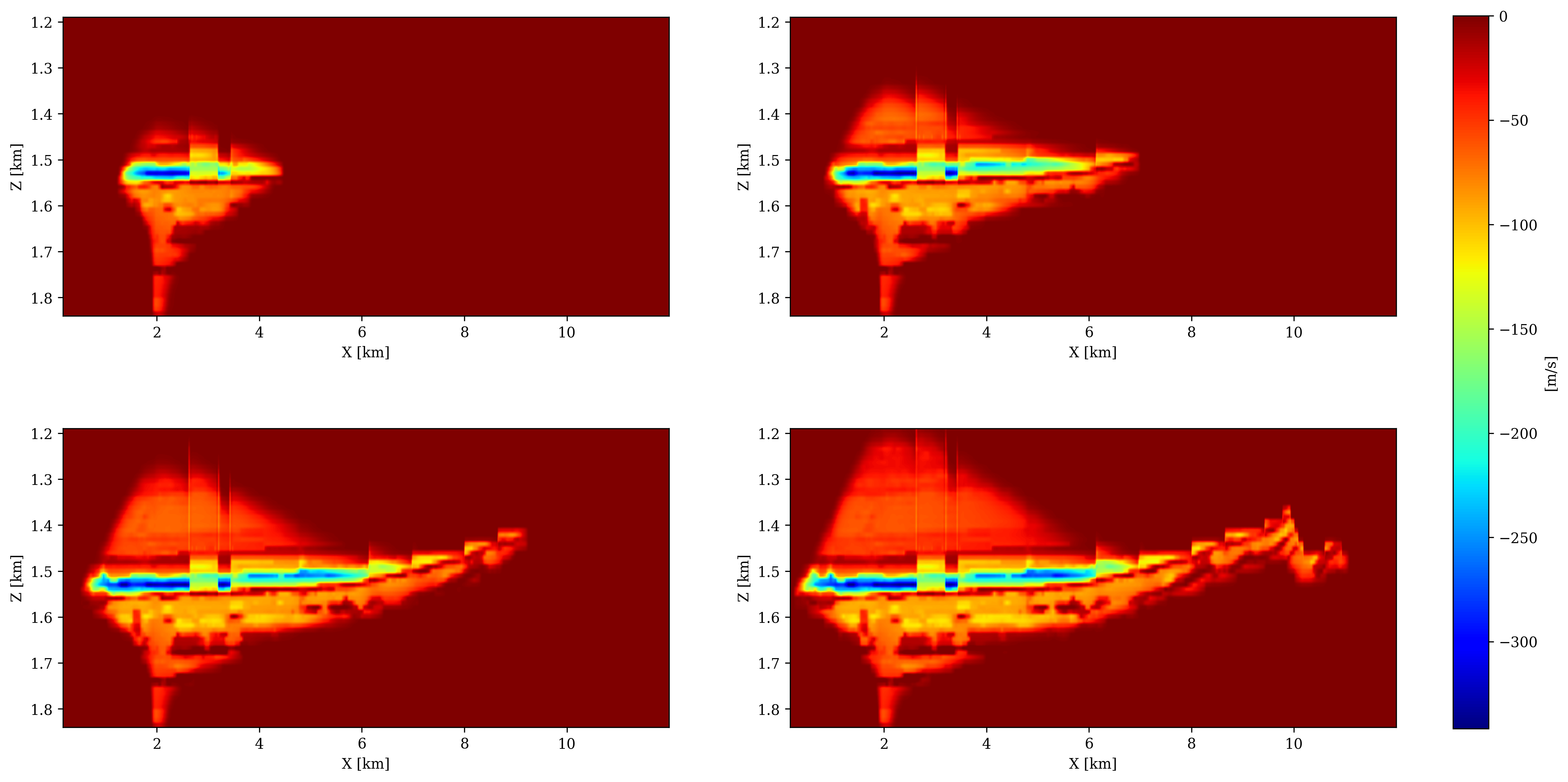
We use the open-source software FwiFlow (D. Li et al., 2020) to numerically simulate the growth of the CO2 plume by solving the partial differential equations for two-phase flow for a period of \(60\) years with a time step of \(20\) days and a grid spacing of \(25\)m. While our numerical simulations are in 2D, we assume the permeability model to extend by \(1.6\) km in the third (perpendicular) direction. The reservoir is initially filled with saline water, with a density of \(1.053\mathrm{g/cm}^3\) and a viscosity of \(1.0\) centipoise (cP). We inject CO2 at a constant rate of \(7\) Mt/y for \(60\) years, amounting to a total of \(420\) million metric tons. During the injection, we assume the supercritical CO2 to have a density of \(776.6 \mathrm{g/cm}^3\) and a viscosity of \(0.1\)cP suggested by (D. Li et al., 2020) and the Strategic UK CCS Storage Appraisal Project. This two-phase flow simulation provides us with a map of the CO2 concentration (in percentage) at the aformentioned time steps. We adopt the patchy saturation model (Avseth et al., 2010; D. Li et al., 2020) to convert these CO2 concentrations to decreases in bulk moduli and then to decreases in compressional wavespeeds, which are included in Figure 2. From this figure, we can see how the plume develops over time under influence of buoyancy and the production well to the right. We also observe that the plume gives rise to a difference in p-wavespeed between \(50\)m/s to \(300\)m/s, which should in principle be detectable via seismic monitoring.

Time-lapse data acquisition

We collect five surveys over a period of \(60\) years, with a baseline survey conducted before CO2 injection starts, followed by \(4\) monitor surveys taken after \(\{15,30,45,60\}\) years of injection. We propose a low-cost sparse non-replicated acquisition scheme with compressive sensing, capable of producing time-lapse seismic data with a high degree of repeatability without relying on replicating the surveys. To keep the costs down, we work with relatively sparsely sampled ocean bottom hydrophones connected to underwater buoys located above the ocean bottom. Compared to ocean bottom nodes, this type of acquisition avoids picking up coherent noise related to interface waves while it shares the advantage of being static and therefore highly replicable. To avoid aliasing, we jitter sample (F. J. Herrmann and Hennenfent, 2008) the receiver positions of \(64\) hydrophones located at a depth of \(120\)m with an average spacing of \(250\)m horizontally. To reduce the costs on the source side, we propose non-replicated continuous simultaneous source shooting, which after deblending (C. Li et al., 2013; Xuan et al., 2020) yields \(1272\) sources with a dense source sampling of \(12.5\)m horizontally. To mimic the challenges related to active-source acquisition, we vary for each survey the tow-depth of sources uniformly randomly from \(5\)m to \(15\)m. We also apply random horizontal shifts varying uniformly in a range of \(-6\)m to \(6\)m, between sources in the different surveys. Since the receivers are coarsely sampled, we employ source-receiver reciprocity during imaging to further reduce computational costs.

Time-lapse monitoring with the joint recovery model

As stated earlier, we assume to have access to kinematically correct background velocity models \(\{\mathbf{\overline{m}}\}_{j=1}^n\). To demonstrate what is in principle achievable under ideal wave-physics, we generate linear data for each vintage via \(\mathbf{\delta d}_j=\nabla\mathcal{F}_j(\mathbf{\overline{m}_j}),\, j=1\cdots n_v\). We implemented both inversion schemes with JUDI – the Julia Devito Inversion framework (Witte et al., 2019a). This open-source package uses the highly optimized time-domain finite-difference propagators of Devito (Luporini et al., 2020; Louboutin et al., 2019). We use a grid spacing of \(10\)m during the wave-equation simulations and a Ricker wavelet with a peak frequency of \(25\)Hz. Despite committing the inversion crime by generating data with the demigration operator, our monitoring problem is complicated by a rather complex but realistic geology (shown in Figure 1) and by the fact that the sampling is coarse on the receiver site and not replicated at the source site. To increase realism, we also use a random trace estimation technique during imaging. During random trace estimation, memory use is reduced drastically, a prerequisite for scaling our approach to \(3\)D. Using the open-source software TimeProbeSeismic.jl, we chose \(32\) random probing vectors to approximate our gradient calculations, which leads to noisy imaging artifacts. We refer to Louboutin and Herrmann (2021) and to the proceedings of this conference for further details.

Independent recovery

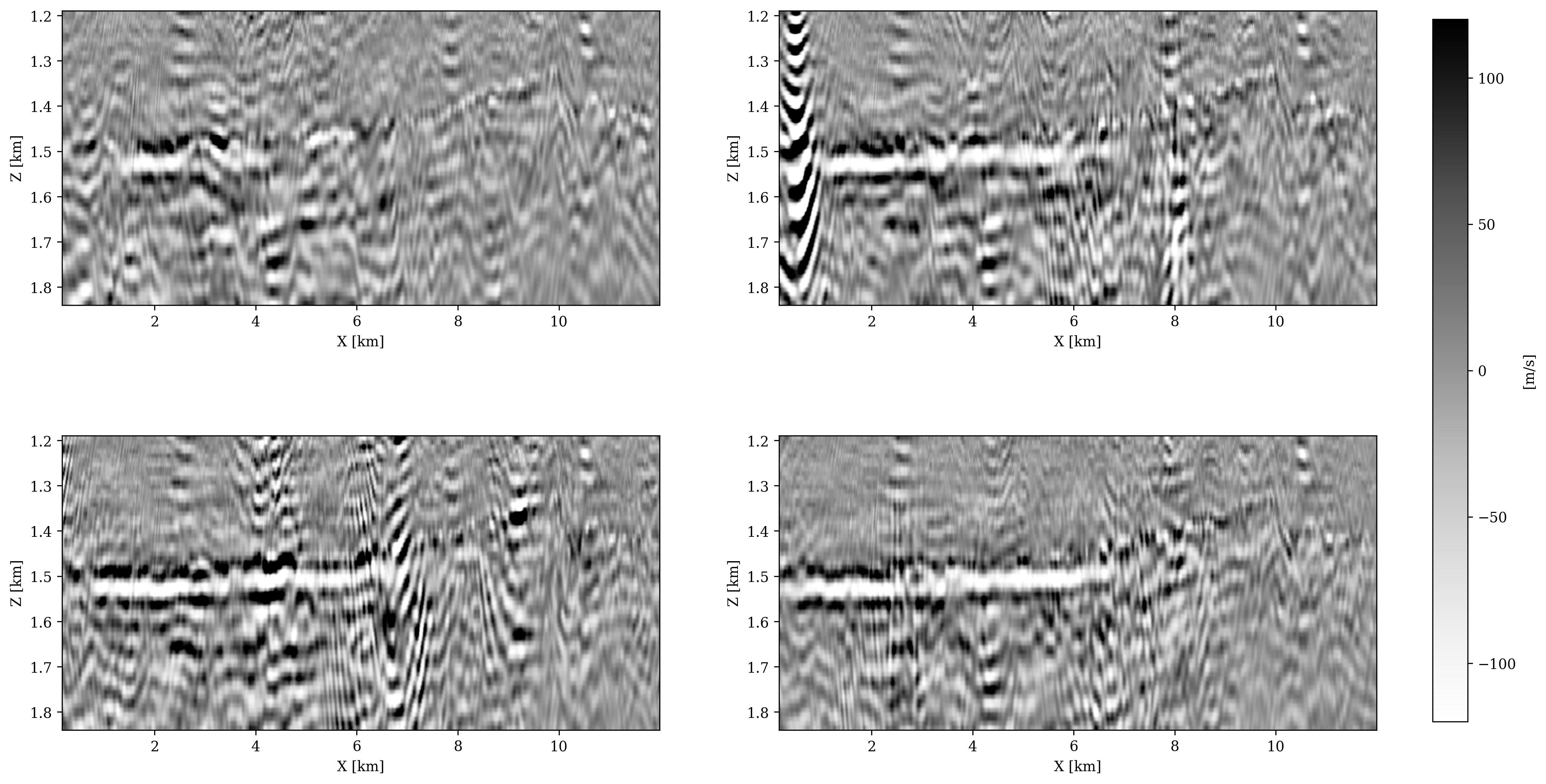
We first recover the velocity perturbations in each vintage independently. During each Bregman iteration, we randomly select eight shots without replication during imaging, while we select \(16\) during the first iteration to build up a good starting image. We use the suggested steplength of Lorenz et al. (2014) and the \(90\)th percentile of \(|\mathbf{u}_k|\) at the first iteration as the threshold \(\lambda\). For each vintage, we do \(23\) Bregman iterations, which amounts to three data passes. To observe the growth of the CO2 plume seismically, we plot the differences of the recovered images for each monitor survey with respect to the baseline in Figure 3. These difference are computed via \(\mathbf{x}_j-\mathbf{x}_1\) for \(j=2,\cdots,n_v\) where \(\mathbf{x}_j\) are the images recovered independently. From these images, we observe that time-lapse signal is visible albeit it is weak while the overall image is plagued by strong artifacts, making it difficult to monitor the CO2 plume.

To quantify the degree of repeatability of the time-lapse images, we follow Kragh and Christie (2002) and use the normalized root mean square (NRMS) values defined as \[ \begin{equation} NRMS(\mathbf{x}_1,\mathbf{x}_j)=\frac{200\times RMS(\mathbf{x}_1-\mathbf{x}_j)}{RMS(\mathbf{x}_1)+RMS(\mathbf{x}_j)}, \quad j=2,\cdots,n_v. \label{eq:NRMS} \end{equation} \] By definition, NRMS values range from \(0\) to \(200\) in percentage where a smaller value indicates recovery results are more repeatable, with \(10\) percent as acceptable by today’s best 4D practices. These NRMS values are calculated only using the regions without time-lapse difference.

Joint recovery

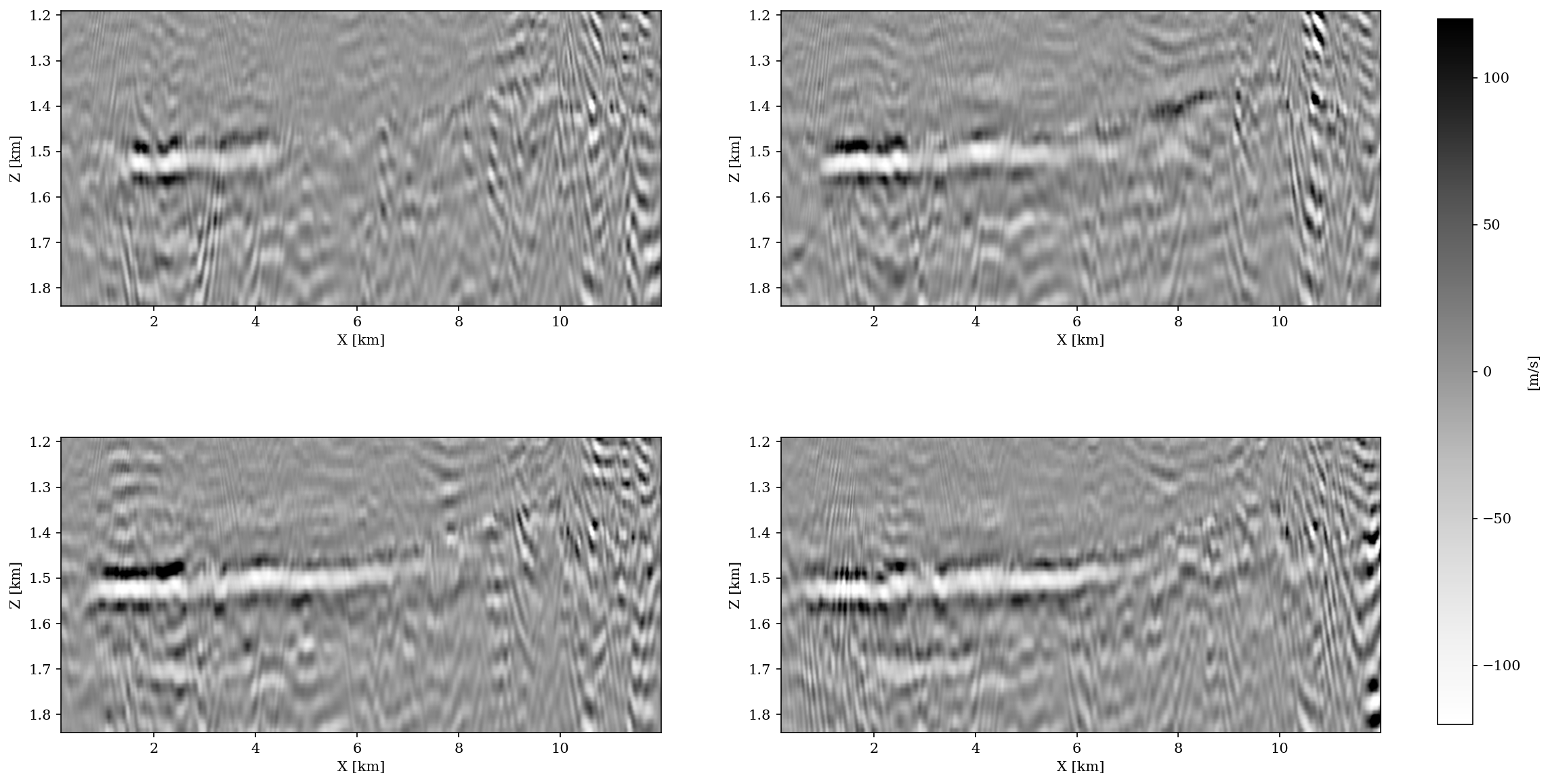
Finally, we recover the common component and innovations jointly via Equation \(\ref{eqjrm}\) with the same number of data passes (same number of PDE solves) and the same random subsets of shots as during the independent recovery. For each vintage, a different threshold \(\lambda_j\) is chosen based on the \(90\)th percentile of the corresponding subset of \(|\mathbf{u}_k|\) at the first iteration. Figure 4 shows the difference plots. Thanks to the JRM, we observe significantly fewer artifacts except for some artifacts in the middle due to overlapping shots during the early iterations, a problem that can easily be fixed. The improved quality of the difference plots is also reflected in the NMRS values, which are now well within the acceptable range. The scripts to reproduce the experiments in this expanded abstract are made available on the SLIM GitHub page https://github.com/slimgroup/Software.SEG2021.

Discussion and conclusions

Time-lapse seismic monitoring of carbon storage and sequestration is difficult due to the fact that the velocity changes induced by the growing CO2 plume are relatively small, making it challenging to detect these changes seismically especially when the surveys are poorly sampled and not replicated. By using the joint recovery model, we demonstrably overcome this problem by producing significant improvements in the difference plots associated with a realistic 60 year sequestration scenario. While similar improvements by the joint recovery model have been reported in the literature, the benefit of this approach has not yet been demonstrated for multiple monitor surveys. Neither has this model been used to monitor the development of a CO2 plume in a realistic geological setting in the North Sea that is currently being considered as a site for CO2 sequestration. While these initial results yielding NMRS values of \(10\)% on average are encouraging, many challenges remain in the development of a low-cost 3D seismic monitoring system designed to control and optimize the CO2 sequestration while minimizing its risk.

Acknowledgement

We would like to thank Charles Jones for the constructive discussion and thank BG Group for providing the Compass model. The CCS project information is taken from the Strategic UK CCS Storage Appraisal Project, funded by DECC, commissioned by the ETI and delivered by Pale Blue Dot Energy, Axis Well Technology and Costain. The information contains copyright information licensed under ETI Open Licence. This research was carried out with the support of Georgia Research Alliance and partners of the ML4Seismic Center.