Transfer learning in large-scale ocean bottom seismic wavefield reconstruction

Mi Zhang\(^{1,3}\), Ali Siahkoohi\(^{2}\), and Felix J. Herrmann\(^{1,2}\)
¹School of Earth and Atmospheric Sciences, Georgia Institute of Technology,
²School of Computational Science and Engineering, Georgia Institute of Technology,
³State Key Laboratory of Petroleum Resources and Prospecting, China University of Petroleum - Beijing

Abstract

Achieving desirable receiver sampling in ocean bottom acquisition is often not possible because of cost considerations. Assuming adequate source sampling is available, which is achievable by virtue of reciprocity and the use of modern randomized (simultaneous-source) marine acquisition technology, we are in a position to train convolutional neural networks (CNNs) to bring the receiver sampling to the same spatial grid as the dense source sampling. To accomplish this task, we form training pairs consisting of densely sampled data and artificially subsampled data using a reciprocity argument and the assumption that the source-site sampling is dense. While this approach has successfully been used on the recovery monochromatic frequency slices, its application in practice calls for wavefield reconstruction of time-domain data. Despite having the option to parallelize, the overall costs of this approach can become prohibitive if we decide to carry out the training and recovery independently for each frequency. Because different frequency slices share information, we propose the use the method of transfer training to make our approach computationally more efficient by warm starting the training with CNN weights obtained from a neighboring frequency slices. If the two neighboring frequency slices share information, we would expect the training to improve and converge faster. Our aim is to prove this principle by carrying a series of carefully selected experiments on a relatively large-scale five-dimensional data synthetic data volume associated with wide-azimuth 3D ocean bottom node acquisition. From these experiments, we observe that by transfer training we are able t significantly speedup in the training, specially at relatively higher frequencies where consecutive frequency slices are more correlated.

Introduction

In seismic exploration, the complex and variable marine environment brings about a unique set set of challenges to data acquisition. Because we can safely assume that sources are sampled densely, by relying on existing work on randomized marine acquisition (Kumar et al., 2015b; Cheng and Sacchi, 2015), our acquisition productivity is dominated by attainable levels of sparsity in the distribution of Ocean Bottom Nodes or Cables (OBN, OBC) without sacrificing the overall quality of long-offset multi-azimuth data. Compared to other acquisition methods, OBNs offer the most flexibility to deliver on this promise but this comes with the challenge that we need to control costs deploying OBNs by sampling the receivers extremely sparsely (at least \(10\times\) subsampled).

This large degree of subsampling challenges most existing wavefield reconstruction techniques that do not, either explicitly as in matrix or tensor completion (Silva and Herrmann, 2014; Kumar et al., 2015a; López et al., 2016) or implicitly as in recent work by Siahkoohi et al. (2019a), leverage correlations that exist in monochromatic frequency slices across the full survey area. The reason of this lies in the fact many approaches (Oropeza and Sacchi, 2011) rely on working in small upto five dimensional windows where long-range correlations that exist in seismic data volumes are ignored limiting their wavefield reconstruction performance for wide-azimuth data. By working with monochromatic data from across the whole survey, wide-azimuth wavefield recovery is feasible for high degrees of subsampling as recently demonstrated by Kumar et al. (2015a), López et al. (2016), and later Zhang et al. (2019). In this work, explicit use is made during the recovery of redundancies within monochromatic data that manifests itself by the fact seismic data can be approximated in low-rank factored form when organized in permuted form by lumping together sources/receivers in \(x\) and \(y\) directions rather than combining source \(x\) and source \(y\) and receiver \(x\) and receiver \(y\). Because fully sampled frequency slices are never formed explicitly, this approach has successfully been applied to industry-scale problems (Kumar et al., 2015a) for the low- to mid-frequency ranges. More accurate wavefield reconstruction at higher frequencies has recently been made possible (Zhang et al., 2019) via a recursive technique that sweeps from low to high frequencies and where factorizations of neighboring (often at lower temporal frequency) frequency slices are used in the recovery of the current frequency slice. This weighting scheme is successful when neighboring frequency slices have information in common with the current frequency slice and recurrent application of this principle has resulted in improvements of wavefield recovery at high frequencies from severely subsampled data.

While (weighted) factored matrix completion techniques have been mainly responsible for full-azimuth wavefield reconstruction from severe subsampling, the low-rank factored approach is somewhat limited because it essentially relies on a shallow (one layer) encoder-decoder (linear)neural network—i.e., the low-rank factors can be thought as neural net encoders decoders. However, from recent successes in machine learning we know that deep convolutional neural networks (CNNs) are capable of capturing more intricate relationships in the data. Judged by the early success of Siahkoohi et al. (2019a), we ague that relationships among the different gathers are captured implicitly by training a Generative Adversarial Network (GAN, Goodfellow et al., 2014) on pairs of fully sampled and subsampled monochromatic single-receiver frequency slices. Compared to the earlier mentioned matrix-completion approach, the latter approach is fundamentally nonlinear during which similarities that live within the data are encoded in the weights of network during training.

While GAN based wavefield reconstruction (Siahkoohi et al., 2018, 2019a) can lead to high-quality reconstructions, its computational costs, and therefore performance, can become an issue especially when we move to higher frequencies. This problem is exacerbated by the fact that each frequency slice is treated independently—i.e., we train and reconstruct each frequency slice separately. We present a method that overcomes this problem by exploiting frequency-to-frequency similarities, in addition to spatial redundancies that live across the monochromatic survey as a whole. As during wavefield recovery with weighted factorizations, we use information from neighboring frequency slices to inform training of the GANs for the different frequencies through transfer training (Yosinski et al., 2014; Siahkoohi et al., 2019b). We base this choice for transfer training on positive experiences we have had using this technique in different areas of seismic data processing and modeling (Siahkoohi et al., 2019b). In these scenarios, transfer learning significantly improved the wavefield reconstruction quality while reducing training costs, specially at relatively higher frequencies where consecutive frequency slices are more correlated.

Our paper is organized as follows. First, we discuss how to use source-receiver reciprocity to construct training and testing data. Second, we briefly introduce Generative Adversarial Networks (GANs, Goodfellow et al., 2014). Next, we explain how to use transfer learning to finetune CNNs that are trained on neighboring frequencies to reduce training costs. Finally, we demonstrate the performance of the proposed method compared to state-of-the-art methods on a large-scale 5D synthetic dataset.

Extracting training pairs from data

In the ocean bottom acquisition geometry discussed in this work, the sources are assumed to be fully-sampled and the receivers are severely subsampled. For this reason for each recorded receiver in the field, the corresponding single-receiver frequency slice is fully sampled. On the other hand, all single-source frequency slices are subsampled because of the sparse OBN sampling.

We train our network to reconstruct monochromatic seismic data by feeding it pairs of artificially subsampled (with a different subsampling mask for each iteration of the training) and fully sampled single-receiver frequency slices. During testing, the trained CNN is used to recover missing values in single-source frequency slices—i.e., information in missing receivers. While not used explicitly, we made in this approach use of reciprocity during training because we worked with receiver gathers with dense source sampling.

Network architecture and optimization

During training of a GAN, the CNN, \(\mathcal{G}_{\theta}\), which performs the wavefield reconstruction, is coupled with an additional CNN, the discriminator, \(\mathcal{D}_{\phi}\), that learns to distinguish between fully-sampled frequency slices and the ones that have been recovered by \(\mathcal{G}_{\theta}\). To enforce the relationship between each specific pair of subsampled and fully-sampled frequency slices, we include an additional \(\ell_1\)-norm misfit term weighted by \(\lambda\) (Isola et al., 2017). We use the following objective function for training GANs with input-output pairs: \[ \begin{equation} \begin{aligned} &\ \min_{\theta} \mathop{\mathbb{E}}_{\mathbf{X}\sim p(\mathbf{X})} \left [ \left (1-\mathcal{D}_{\phi} \left (\mathcal{G}_{\theta} (\mathbf{M} \odot \mathbf{X}) \right) \right)^2 + \lambda \left \| \mathcal{G}_{\theta} (\mathbf{M} \odot \mathbf{X})-\mathbf{X} \right \|_1 \right ] ,\\ &\ \min_{\phi} \mathop{\mathbb{E}}_{\mathbf{X}\sim p(\mathbf{X})} \left [ \left( \mathcal{D}_{\phi} \left (\mathcal{G}_{\theta}(\mathbf{M} \odot \mathbf{X}) \right) \right)^2 \ + \left (1-\mathcal{D}_{\phi} \left (\mathbf{X} \right) \right)^2 \right ], \end{aligned} \label{adversarial-training} \end{equation} \] where \(\mathbf{M}\) is the training mask, \(\odot\) element-wise multiplication, and the expectations are approximated with the empirical mean computed over \(\mathbf{X}_i, \ i = 1,2, \ldots , N_R\)-–i.e., fully-sampled single-receiver frequency slices drawn from the probability distributions \(p (\mathbf{X})\). As proposed by Johnson et al. (2016), we use a ResNet (He et al., 2016) for the generator \(\mathcal{G}_{\theta}\) and we follow Isola et al. (2017) for the discriminator \(\mathcal{D}_{\phi}\) architecture. We set the hyper-parameter \(\lambda\) as 1000 to balance generator’s tasks for fooling the discriminator and mapping specific pairs \((\mathbf{M} \odot \mathbf{X}_i,\, \mathbf{X}_i)\) to each other (Isola et al., 2017). Solving the optimization objective \(\ref{adversarial-training}\) is typically based on Stochastic Gradient Descent (SGD) or one of its variants (Goodfellow et al., 2016; Bottou et al., 2018).

Transfer learning between correlated frequencies

Transfer learning involves utilizing the knowledge a neural network has gained during pretraining in order to perform another but related task (Pan and Yang, 2010; Bengio, 2012; Siahkoohi et al., 2019b). In the proposed deep-learning-based wavefield reconstruction framework, we finetune weights of the CNN trained to reconstruct a neighboring frequency component to reconstruct the slices of the current frequency component. In case neighboring frequency slices are similar, this may speed up the training compared to training a CNN from scratch.

Since the performance of transfer learning depends on the similarity between tasks (Ammar et al., 2014; Dwivedi and Roig, 2019), it is best to perform correlation analysis before transfer learning. To make this qualitative statement more quantitative, we calculate the smallest principal angles between row (or column) subspaces of two frequency slices (Zhang et al., 2019). Interested readers can refer to Eftekhari et al. (2018) for an extensive overview of the calculation. Small angles indicate a high correlation between two slices. According to this calculation, the smallest angle value of row subspaces is \(0.11\) radian between \(9.33\) Hz and \(9.66\) Hz, whereas it is \(0.08\) radian between \(14.33\) Hz and \(14.66\) Hz. Similarly the smallest angle value of column subspaces is \(0.17\) radian between \(9.33\) Hz and \(9.66\) Hz, whereas it is \(0.10\) radian between \(14.33\) Hz and \(14.66\) Hz. Notwithstanding the fact that these angles are obtained based on a linear factorization of the data, these values partially support the fact that the correlation between two adjacent frequencies \(14.33\) and \(14.66\) Hz is slightly higher than that between two non-adjacent frequencies \(9.33\) and \(14.66\) Hz. For this reason, we expect to see transfer learning to perform slightly more efficiently when applied to finetune weights of the CNN trained to reconstruct \(14.33\) frequency slices to reconstruct the \(14.33\) frequency slices.

Numerical Experiments

To explore the reconstruction ability of the proposed method, we apply it on a 5D synthetic dataset simulated to a portion of BG Compass model with highly sparse receivers (\(90\%\) of receivers are randomly missing) and compare it with the low-rank matrix completion methods (Kumar et al., 2015a; Zhang et al., 2019). The geometry is composed of a \(172 \times 172\) periodic grid of sources and a \(172 \times 172\) periodic grid of receivers, both with \(25\) m spatial sampling interval in both \(x\) and \(y\) directions. We perform 1D fast Fourier transform (FFT) to transform the seismic data from the time domain to the frequency domain and then extract monochromatic \(9.33\), \(9.66\), \(14.33\), and \(14.66\) Hz frequency components to showcase our method. For different frequency components, we construct the corresponding training and test sets according to the previously mentioned permutation. Then we pretrain a randomly initialized CNN on all extracted monochromatic frequency slices. Next, we employ transfer learning and use the CNN weights trained to reconstruct monochromatic seismic slices at \(9.33\) and \(14.33\) Hz as an initial guess to train CNNs to reconstruct \(9.66\) and \(14.66\) Hz data. As mentioned before, during training (and transfer learning), we change the training mask at every epoch, hence, each training pair is only used once during optimization. Therefore, the performance of the CNN over testing dataset (or validation set) can be accurately approximated using the training data set. For this reason, we safely calculate the SNR over training pairs at during training as the metric to assess the reconstruction capability of network on test data.

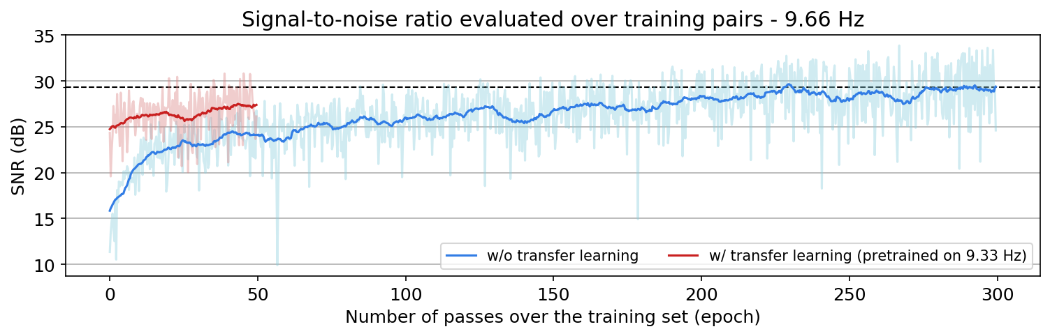
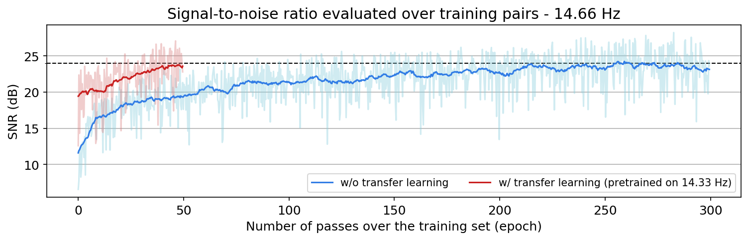
Figure 1a shows a comparison between \(9.66\) Hz frequency slice reconstruction SNRs, evaluated over training data during training, using the original deep-learning based method (light-blue)—i.e., training a randomly initialized, and result obtained by transfer learning (light-red)—i.e., transferring a CNN pretrained to reconstruct \(9.33\) Hz slices frequency slices to reconstruct 14.66 frequency slices. Similarly, Figure 1 shows the sampe comparison between for \(14.66\) Hz when we either train a randomly initialized CNN or apply transfer learning using a CNN trained to reconstruct \(14.33\) Hz data. Dark colors indicate a running average over light curves to clarify the overall trend. We can see that over \(50\) epochs, the average SNR of transfer learning of the CNN pretrained to reconstruct \(14.33\) frequency slices is always higher than that of the CNN directly trained from scratch to reconstruct \(14.66\)frequency slices. We make a similar observation in Figure 1a as well, except that transfer learning needs more than \(50\) epochs to obtain same reconstruction SNR as the result without transfer learning. This observation coincides with our expectation that transfer learning is more effective when applied to more correlated tasks—i.e., when neighboring frequency slices are more correlated. We also observed that using transfer learning to reconstruct a neighboring frequency can significantly speed up the the training, specially when consecutive frequency slices are more correlated.

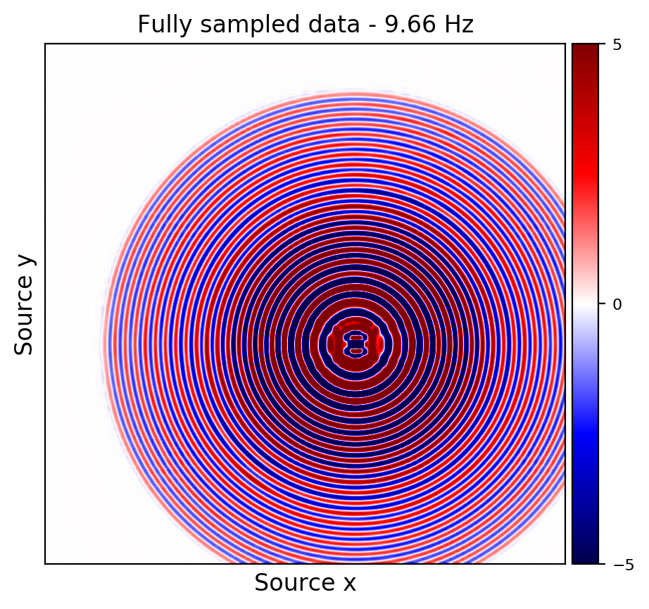
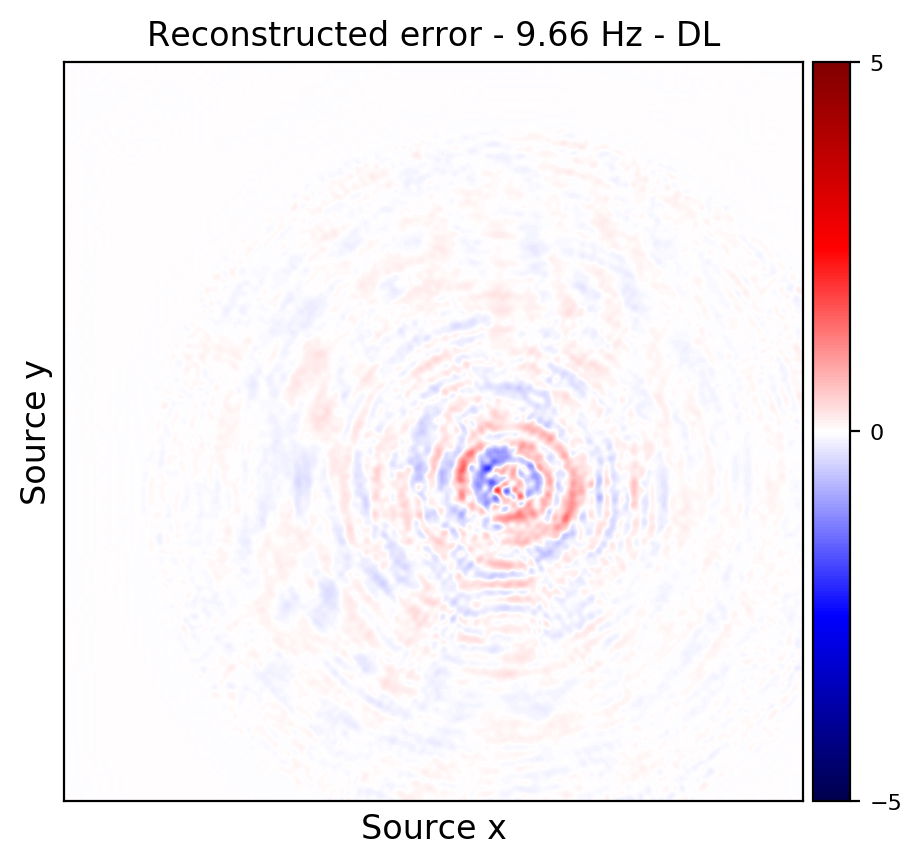
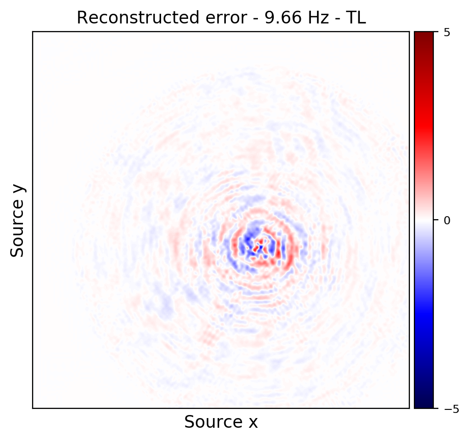
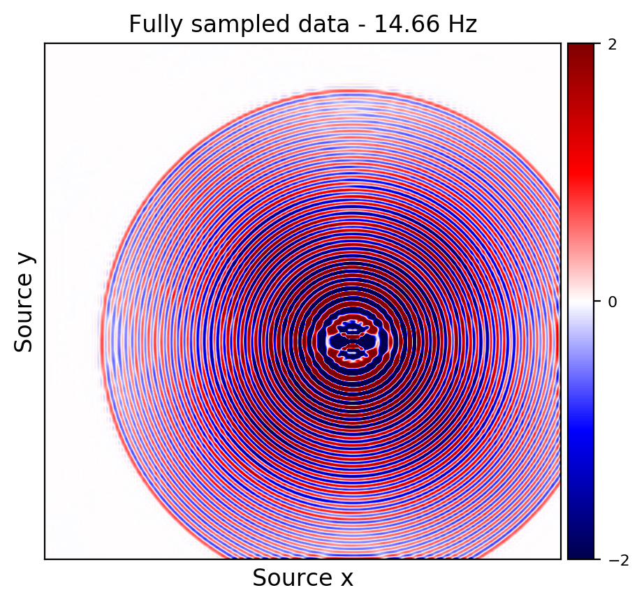
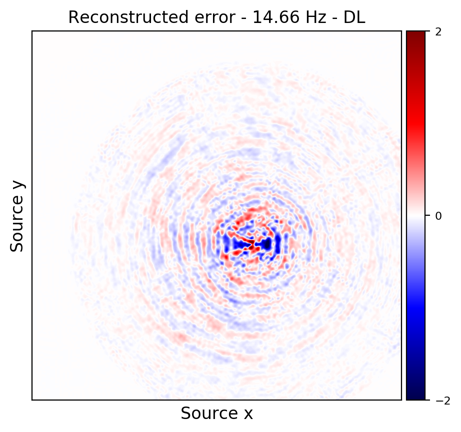
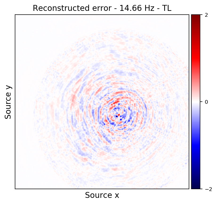
Figures 2a and 2d depict ground truth \(9.66\) and \(14.66\) Hz single-receiver frequency slices for a receiver that we have assumed is missing in the observed data. Figures 2b and 2c show the reconstruction error obtained by training a randomly initialized CNN and utilizing transfer learning to recover \(9.66\) Hz data, respectively. Similar figures for \(14.66\) can be seen in Figures 2e and 2e. As it can be seen, transfer learning has been able to recover the slices with similar quality, using much less computational cost. However, transfer learning does a better job at recovering \(14.66\) Hz data, which coincides with our expectation given higher correlations among consecutive frequency slices at higher frequencies.

Conclusions

In this work, we proposed to utilize transfer learning to improve the training efficiency of our deep learning framework for seismic ocean bottom wavefield reconstruction. Considering the similarities between reconstruction tasks for frequency slices at neighboring frequencies, we transfer the knowledge learned by the neural network for one frequency to the other frequency. Our experiments on the 5D synthetic data indicate that the knowledge transferred from adjacent frequencies is reliable as long as the frequency slices share information. We found that that is typically the case for higher frequencies that share more information. We argue that this could be attributed to the fact that at low frequencies the monochromatic slices are more orthogonal and therefore share less information. Compared to our original deep-learning based method, the proposed framework can speed up the training six fold while improving the reconstruction performance.

Related materials

In order to facilitate the reproducibility of the results herein discussed, a PyTorch (Paszke et al., 2019) implementation of this work is made available on the GitHub.