Weak deep priors for seismic imaging

Ali Siahkoohi, Gabrio Rizzuti, and Felix J. Herrmann
School of Computational Science and Engineering,
Georgia Institute of Technology

Introduction

Linearized seismic imaging involves an inconsistent, ill-conditioned linear inverse problem due to presence of shadow zones and complex structures in the subsurface, coherent linearization errors, and noisy data. Due to nonuniqueness, using prior information as regularization is essential. This particular choice is crucial because it typically affects the final result. Conventional methods mostly rely on handcrafted and unrealistic priors, such as a Gaussian or Laplace distributed model parameters (in the physical or in a transform domain). These simplifying assumptions, while being practical, negatively bias the outcome of the inversion.

Recent proposals (Lempitsky et al., 2018; Cheng et al., 2019; Gadelha et al., 2019; Liu et al., 2019; Y. Wu and McMechan, 2019; Shi et al., 2020; Siahkoohi et al., 2020) make use of convolutional neural networks (CNN) as a prior. Specifically, Siahkoohi et al. (2020) reparameterize the unknown reflectivity model by a CNN and impose a Gaussian prior on its weights. These authors show that the combination of the functional form of a CNN and a Gaussian prior on its weights is a suitable prior for seismic imaging. However, since every update to CNN weights requires the action of the forward operator and its adjoint, tuning randomly initialized CNN weights need many stochastic optimization steps. In seismic imaging, computing the action of the forward operator—i.e., linearized Born scattering operator, and its adjoint is computationally expensive, which might limit the application of deep priors.

We propose the weak deep prior, a computationally convenient formulation that relaxes deep priors. Instead of reparameterizing the unknowns with CNNs, we let the unknown reflectivity to be distributed according to a Gaussian distribution centered at the CNN network output. Next, we jointly solve for the reflectivity model and CNN weights. This formulation decouples the forward operator with the CNN, allowing for fast and forward-operator free updates of CNN weights, while partially keeping the advantages of the deep prior. The proposed formulation additionally allows for imposing handcrafted or physical hard constraints on the unknowns, which is often not feasible when imposing deep priors (Herrmann et al., 2019).

In general, numerous efforts involve the incorporation of ideas from deep learning in seismic processing and inversion (Ovcharenko et al., 2019; Rizzuti et al., 2019; Siahkoohi et al., 2019a, 2019b, 2019c; Sun and Demanet, 2019; Z. Zhang and Alkhalifah, 2019). Deep prior itself have been utilized by Liu et al. (2019) to perform seismic data reconstruction. Y. Wu and McMechan (2019) propose to pretrain a randomly initialized CNN before reparameterizing the velocity model in the context of Full-Waveform Inversion. Shi et al. (2020) use the deep priors in the context of denoising. Finally, Siahkoohi et al. (2020) proposes a deep-prior based Bayesian framework for seismic imaging and perform uncertainty quantification.

Our work is organized as follows. We first introduce the original concept of deep prior and how it can be integrated in seismic imaging. Next, we develop the weak deep prior framework and the associated optimization problem. We conclude by showcasing the proposed method using a synthetic example involving a 2D portion of a real migrated image of the 3D Parihaka dataset (Veritas, 2005; WesternGeco., 2012) in the presence of strong noise.

Seismic imaging

Seismic imaging is the problem of estimating the short-wavelength structure of the Earth’s subsurface, denoted by \(\delta \mathbf{m}\) given data recorded at the surface, \(\delta \mathbf{d}_{i}, \ i = 1,2, \cdots , N\), where \(N\) is the number of shot records. Besides observed data, this inverse problem requires a smooth background squared-slowness model, \(\mathbf{m}_0\), and estimated source signatures, \(\mathbf{q}_i\). When noise in the data can be approximated by a zero-mean Gaussian random variable, \(\ell_2\)-norm data discrepancy defines the likelihood function (Tarantola, 2005). Assuming the noise covariance is \(\sigma^2 \mathbf{I}\), we can write the negative log-likelihood of the observed data as follows: \[ \begin{equation} \begin{aligned} &\ - \log p_{\text{like}} \left ( \left \{ \delta \mathbf{d}_{i} \right \}_{i=1}^N \normalsize{|}\delta \mathbf{m} \right ) = -\sum_{i=1}^N \log p_{\text{like}} \left ( \delta \mathbf{d}_{i} \normalsize{|}\delta \mathbf{m} \right ) \\ &\ = \frac{1}{2 \sigma^2} \sum_{i=1}^N \|\delta \mathbf{d}_i- \mathbf{J}(\mathbf{m}_0, \mathbf{q}_i) \delta \mathbf{m}\|_2^2 \quad + \underbrace {\text{const}}_{\text{Ind. of } \delta \mathbf{m}}. \\ \end{aligned} \label{nll} \end{equation} \] In these expressions, \(p_{\text{like}}\) denotes the likelihood probability density function, and \(\mathbf{J}\) is the linearized Born scattering operator. The maximum likelihood estimate (MLE), denoted by \(\widehat{\delta \mathbf{m}}_{\text{MLE}}\), is obtained by minimizing the negative-log likelihood defined in Equation \(\ref{nll}\) with respect to \(\delta \mathbf{m}\). Notoriously, MLE estimators tend to produce imaging artifacts. To address this issue, we discuss a special kind of prior based on neural networks: the so-called deep priors.

Imaging with deep priors

Parameterizing the unknown variables with a CNN, with a fixed input, has shown promising results in inverse problems (Lempitsky et al., 2018; Cheng et al., 2019; Gadelha et al., 2019; Liu et al., 2019; Y. Wu and McMechan, 2019; Shi et al., 2020; Siahkoohi et al., 2020). In this approach, weights and biases are Gaussian random variables and they are tuned to fit the observed data. The success of this approach hinges on the special structure of the CNN, which tends to favor noise-free looking images. Despite this feature, it should be noted that a stopping criteria is still essential to avoid overfitting the noise in observed data. Notwithstanding this challenge, we propose to parameterize the unknown reflectivity model by a CNN—i.e., \(\delta \mathbf{m} = {g} (\mathbf{z}, \mathbf{w})\), where \(\mathbf{z} \sim \mathrm{N}( \mathbf{0}, \mathbf{I})\) is the fixed input to the CNN and \(\mathbf{w}\) denotes the unknown CNN weights. Imposing a Gaussian prior on \(\mathbf{w}\) with covariance matrix \(\lambda^{-2}\mathbf{I}\) allows us to formulate the negative log-posterior distribution for \(\mathbf{w}\) as follows: \[ \begin{equation} \begin{aligned} &\ p_{\text{post}} \left ( \mathbf{w} \normalsize{|} \left \{ \delta \mathbf{d}_{i} \right \}_{i=1}^N \right ) \propto \left [ \prod_{i=1}^{N} p_{\text{like}} \left ( \delta \mathbf{d}_{i} \normalsize{|}\mathbf{w} \right ) \right ] p_{w} \left ( \mathbf{w} \right ), \\ &\ \text{where} \quad p_{w} \left ( \mathbf{w} \right ) = \mathrm{N}(\mathbf{w} \normalsize{|} \mathbf{0}, \lambda^{-2}\mathbf{I}). \\ \end{aligned} \label{deep-prior} \end{equation} \] In the equation above, \(p_{w}\) and \(p_{\text{post}}\) denote the prior and posterior probability density functions, respectively. The maximum a posteriori estimator (MAP), denoted by \(\widehat{\mathbf{w}}_{\text{deep}}\), is obtained by maximizing Equation \(\ref{deep-prior}\) with respect to \(\mathbf{w}\).

As stated before, there are two challenges in employing deep priors in seismic imaging. The first challenge is finding a stopping criteria while maximizing the posterior in Equation \(\ref{deep-prior}\) to prevent noise overfit. Siahkoohi et al. (2020) propose to perform stochastic gradient Langevin dynamics (SGLD, Welling and Teh, 2011) steps to obtain samples from this posterior distribution. Using these samples, these authors approximate the conditional mean estimator, which prevents overfitting and at the same time, yields a seismic image that has less imaging artifacts compared to the MAP estimator. However, sampling the posterior is a challenging feat in and of itself and is outside of the scope of this discussion. Another challenge associated with deep-prior based imaging is the number of iterations needed to optimize the CNN weights. Unless the CNN is pretrained, its weights are initialized randomly, hence, solving for \(\mathbf{w}\) requires many iterations involving the seismic modeling operator and its adjoint and may not be computationally practical. Unfortunately, unlike other imaging modalities, such as medical imaging, we generally do not have access to detailed information on the subsurface. This limits the scope of the pretraining phase, which in turn might adversely bias the outcome of the inversion, and contradicts the premises of this work. In the next section, we introduce our proposed method and discuss how to address the computational challenges associated with optimizing the CNN’s randomly initialized weights, while keeping the advantages of the deep-prior based imaging.

Imaging with weak deep prior

The deep-prior based imaging problem can equivalently be casted as the following constrained optimization problem: \[ \begin{equation} \begin{aligned} &\ \mathop{\rm arg\,min}_{\delta \mathbf{m},\, \mathbf{w}}\frac{1}{2 \sigma^2} \left [ \sum_{i=1}^N \|\delta \mathbf{d}_i- \mathbf{J}(\mathbf{m}_0, \mathbf{q}_i) \delta \mathbf{m} \|_2^2 + \frac{\lambda^2}{2} \| \mathbf{w} \|_2^2 \right ] \\ &\ \text{subject to}\quad \delta \mathbf{m}=g (\mathbf{z}, \mathbf{w}), \\ \end{aligned} \label{nlp-deep-prior} \end{equation} \] where we restrict the feasible model to the output of \(g (\mathbf{z}, \mathbf{w})\). To address the computational challenge associated with deep-prior based imaging, we propose to relax the constraint in problem \(\ref{nlp-deep-prior}\) and let \(\delta \mathbf{m}\) be a random variable distributed according to a Gaussian distribution centered at \(g (\mathbf{z}, \mathbf{w})\) with covariance matrix \(\gamma^{-2}\mathbf{I}\). We denote the defined prior on \(\delta \mathbf{m}\) as the weak deep prior. By decoupling the forward operator and the CNN weights, observed data becomes conditionally independent from \(\mathbf{w}\), given \(\delta \mathbf{m}\). We can write the joint posterior distribution for \((\delta \mathbf{m},\mathbf{w})\) using the defined prior as follows: \[ \begin{equation} \begin{aligned} &\ p_{\text{post}} \left (\delta \mathbf{m}, \mathbf{w} \normalsize{|} \left \{ \delta \mathbf{d}_{i} \right \}_{i=1}^N \right ) \\ &\ \propto \left [ \prod_{i=1}^{N} p_{\text{like}} \left ( \delta \mathbf{d}_{i} \normalsize{|}\delta \mathbf{m} \right ) \right ] p_{\mathbf{\text{weak}}} \left ( \delta \mathbf{m} \normalsize{|} \mathbf{w} \right )p_{w}(\mathbf{w}), \\ &\ \text{where} \quad p_{\mathbf{\text{weak}}} \left ( \delta \mathbf{m} \normalsize{|} \mathbf{w} \right ) = \mathrm{N}( \delta \mathbf{m} \normalsize{|} g (\mathbf{z}, \mathbf{w}), \gamma^{-2}\mathbf{I}). \\ \end{aligned} \label{weak-deep-prior} \end{equation} \] In Equation \(\ref{weak-deep-prior}\), \(p_{\mathbf{\text{weak}}} \left ( \delta \mathbf{m} \normalsize{|} \mathbf{w} \right )\) denotes the weak deep prior, which is equivalent to a Gaussian distribution centered at \(g (\mathbf{z}, \mathbf{w})\) with covariance matrix \(\gamma^{-2}\mathbf{I}\). \(\gamma\) is a hyperparameter that needs to be tuned. We solve the imaging with weak deep prior problem by minimizing the negative log-posterior defined in Equation \(\ref{weak-deep-prior}\) as follows: \[ \begin{equation} \begin{aligned} \widehat{\delta \mathbf{m}}_{\text{weak}}, \widehat{\mathbf{w}}_{\text{weak}} =\mathop{\rm arg\,min}_{\delta \mathbf{m},\, \mathbf{w}} &\ \left [ \frac{1}{2 \sigma^2} \sum_{i=1}^N \|\delta \mathbf{d}_i- \mathbf{J}(\mathbf{m}_0, \mathbf{q}_i) \delta \mathbf{m} \|_2^2 \right. \\ &\ \left. \ + \ \frac{\gamma^2}{2} \| \delta \mathbf{m} - g (\mathbf{z}, \mathbf{w}) \|_2^2 + \frac{\lambda^2}{2} \| \mathbf{w} \|_2^2 \vphantom{\sum_{i=1}^N} \right ] \\ \end{aligned} \label{nlp-weak-deep-prior} \end{equation} \] where \(\widehat{\delta \mathbf{m}}_{\text{weak}}\) and \(\widehat{\mathbf{w}}_{\text{weak}}\) are the obtained reflectivity and CNN weights by solving the imaging with weak deep prior problem. We consider \(\widehat{\delta \mathbf{m}}_{\text{weak}}\) as the final estimate in this approach. When \(\gamma \rightarrow \infty\), the solution to problem \(\ref{nlp-weak-deep-prior}\) is the same as the solution to problem \(\ref{nlp-deep-prior}\).

In formulation above, updating the parameters \(\mathbf{w}\) does not involve the action of the forward operator, hence, weights of the CNN can be quickly and independently updated. Moreover, the optimization problem \(\ref{nlp-weak-deep-prior}\) offers flexibility to impose any intersection of physical or handcrafted hard constraints, \(\mathcal{C}\), by limiting the search space to \(\delta \mathbf{m} \in \mathcal{C}\) while minimizing the objective with respect to \(\delta \mathbf{m}\), using standard constrained optimization techniques (Peters et al., 2019). In a similar fashion, Herrmann et al. (2019) use a Total-Variation constraint in the context of seismic imaging to jointly solve the imaging problem and train a generative model capable of directly sampling the posterior using the Expectation-Maximization method. As the main contribution of this work, we choose not to utilize hard constraints and focus on the computational aspect of the weak deep prior.

Algorithm and implementation details

To limit the computational cost—i.e., number of wave-equation solves, we use stochastic optimization algorithms to solve the optimization problems \(\ref{nlp-deep-prior}\) and \(\ref{nlp-weak-deep-prior}\). We approximate the negative-log likelihood term (see Equation \(\ref{nll}\)) using a single simultaneous source, made of a Gaussian weighted source aggregate. While we could use stochastic gradient descent algorithm (SGD, Robbins, 2007), we avoid it because of several challenges associated with it. For example, even though SGD’s “noisy” (approximate) gradient is an unbiased estimate of true gradient, its variance is proportional to square of the step size. Therefore, choosing the step size is a trade-off between convergence speed and accuracy. Additionally, SGD updates different components of the unknown with the same step size—i.e., no preconditioning, which is not desirable when the objective has varying sensitivity with respect to different components of the unknowns. Various stochastic optimization algorithms to some extent address these issues by diagonally weighting the gradient by the norm of the past gradients (Duchi et al., 2011) or the (weighted) mean of past squared gradients (Tieleman and Hinton, 2012). We use Adagrad (Duchi et al., 2011) with step size \(2 \times 10^{-3}\) to update \(\delta \mathbf{m}\) while estimating \(\widehat{\delta \mathbf{m}}_{\text{MLE}}\), and when solving optimization problem \(\ref{nlp-weak-deep-prior}\). To update \(\mathbf{w}\), either in optimization problem \(\ref{nlp-deep-prior}\) or \(\ref{nlp-weak-deep-prior}\), we use RMSprop (Tieleman and Hinton, 2012) with step size \(10^{-3}\). We set the step sizes by extensive hyper-parameter tuning. In Algorithm 1, which summarizes our proposed approach, Adagrad and RMSprop are optimization subroutines that given the objective value and the step size, provide an update for \(\delta \mathbf{m}\) and \(\mathbf{w}\), respectively.

Input:
      \(\mathbf{z} \sim \mathrm{N}( \mathbf{0}, \mathbf{I})\): fixed input to the CNN
      \(\lambda, \ \gamma\): trade-off parameters
      \(\sigma^2\): estimated noise variance
      \(T\): stochastic optimization steps for \(\delta \mathbf{m}\)
      \(K\): inner loop stochastic optimization steps for \(\mathbf{w}\)
      \(\eta\), \(\tau\): step sizes to update \(\delta \mathbf{m}\) and \(\mathbf{w}\), respectively
      \(\left \{ \delta \mathbf{d}_{i}, \delta \mathbf{q}_{i} \right \}_{i=1}^N\): observed data and source signatures
      \(\mathbf{m}_0\): smooth background squared-slowness model
      Adagrad: Adagrad algorithm to update \(\delta \mathbf{m}\)
      RMSprop: RMSprop algorithm to update \(\mathbf{w}\)
Initialization:
      Randomly initialize CNN parameters, \(\mathbf{w}\)
      \(\delta \mathbf{m} = \mathbf{0}\)
1. for \(t=1\) to \(T\) do
2.    Randomly sample \((\delta \mathbf{d}, \mathbf{q})\) from \(\left \{ \delta \mathbf{d}_{i}, \mathbf{q}_{i} \right \}_{i=1}^N\)
3.    \(\mathcal{L}(\delta \mathbf{m}) = \frac{N}{2 \sigma^2} \|\delta \mathbf{d}- \mathbf{J}(\mathbf{m}_0, \mathbf{q}) \delta \mathbf{m} \|_2^2 + \frac{\gamma^2}{2} \| \delta \mathbf{m} - g (\mathbf{z}, \mathbf{w}) \|_2^2\)
4.    \(\delta \mathbf{m} \leftarrow\) Adagrad \((\mathcal{L}(\delta \mathbf{m}), \eta)\)
5.    for \(k=1\) to \(K\) do
6.        \(\mathcal{L}(\mathbf{w})= \frac{\gamma^2}{2} \| \delta \mathbf{m} - g (\mathbf{z}, \mathbf{w}) \|_2^2+ \frac{\lambda^2}{2} \| \mathbf{w} \|_2^2\)
7.        \(\mathbf{w} \leftarrow\) RMSprop \((\mathcal{L}(\mathbf{w}), \tau)\)
8.    end for
9. end for
Output: \(\delta \mathbf{m}\)

As mentioned before, the weak deep prior allows for fast updates of the CNN weights (see the inner loop in lines \(5\) – \(8\) of Algorithm 1). However, choosing the number of updates for \(\mathbf{w}\) per each \(\delta \mathbf{m}\) update is a trade-off between reducing computational cost (many \(\mathbf{w}\) updates) and preserving the the deep prior advantages (maintained by employing several \(\mathbf{w}\) updates). In the extreme case, if we update \(\mathbf{w}\) once per \(\delta \mathbf{m}\) update, there is no computational gain compared to the deep-prior based approach. On the other hand, if we solve for \(\mathbf{w}\) after each update to \(\delta \mathbf{m}\)-–i.e., \(\| \delta \mathbf{m} - g (\mathbf{z}, \mathbf{w}) \|_2^2 \simeq 0\), the CNN has almost no effect in the next update for \(\delta \mathbf{m}\). To strike a balance between the number of updates to \(\delta \mathbf{m}\) and \(\mathbf{w}\), we choose to alternatingly take one gradient step for \(\delta \mathbf{m}\) and ten gradient steps for \(\mathbf{w}\).

We use Devito (Luporini et al., 2018; M. Louboutin et al., 2019) to compute matrix-free actions of the linearized Born scattering operator and its adjoint. By integrating these operators into PyTorch, we are able to solve the optimization problems \(\ref{nlp-deep-prior}\) and \(\ref{nlp-weak-deep-prior}\) with automatic differentiation. We follow Lempitsky et al. (2018) for the CNN architecture. We provide more details regarding to our implementation on GitHub.

Numerical experiments

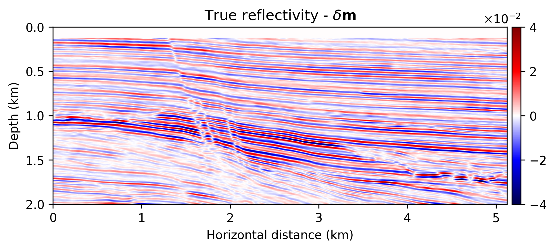
We compare the seismic images obtained by solving problems \(\ref{nlp-deep-prior}\) and \(\ref{nlp-weak-deep-prior}\), when applied to a “quasi” real field data example consisting of a 2D portion of the Kirchoff time migrated 3D Parihaka dataset (see Figure 1a). These imaging results are set as the ground truth for the experiment here discussed. Synthetic data is obtained by applying the linearized Born scattering operator to this “true” reflectivity image. The dataset includes \(205\) shot records sampled with a source spacing of \(25\, \mathrm{m}\) and \(1.5\) seconds recording time. There are \(410\) fixed receivers sampled at \(12.5 \mathrm{m}\) spread across the survey area. The source is a Ricker wavelet with a central frequency of \(30\,\mathrm{Hz}\). To demonstrate the regularization effect of our method, we add a significant amount of noise to the shot records, yielding a low signal-to-noise ratio of the “observed” data of \(-18.01\, \mathrm{dB}\). To limit the computational costs, we mix the shot records according to normally distributed source encodings. By conducting extensive parameter tuning, we set \(\lambda^2 = 2 \times 10^3\) (Equations \(\ref{nlp-deep-prior}\) and \(\ref{nlp-weak-deep-prior}\)) throughout all experiments. We also set \(\sigma^2 = 0.01\) (Equations \(\ref{nll}\), \(\ref{nlp-deep-prior}\), and \(\ref{nlp-weak-deep-prior}\)), which is equal to the variance of the measurement noise. To provide evidence regarding to the computational feasibility of the weak deep prior formulation, we fix the number of passes over the dataset—i.e., we use roughly twice the computational cost of reverse-time migration (computational budget for large-scale least-squares imaging) However, as mentioned before, the deep prior formulation requires more iterations to generate a reasonable image. We use \(15\) passes over the dataset to solve problem \(\ref{nlp-deep-prior}\)-–i.e., to compute \(\widehat{\mathbf{w}}_{\text{deep}}\). Note that taking one gradient step for \(\delta \mathbf{m}\) takes roughly \(60\) times more time than one update of \(\mathbf{w}\), without GPU acceleration. Therefore, we neglect the CNN weights update times in our comparisons.

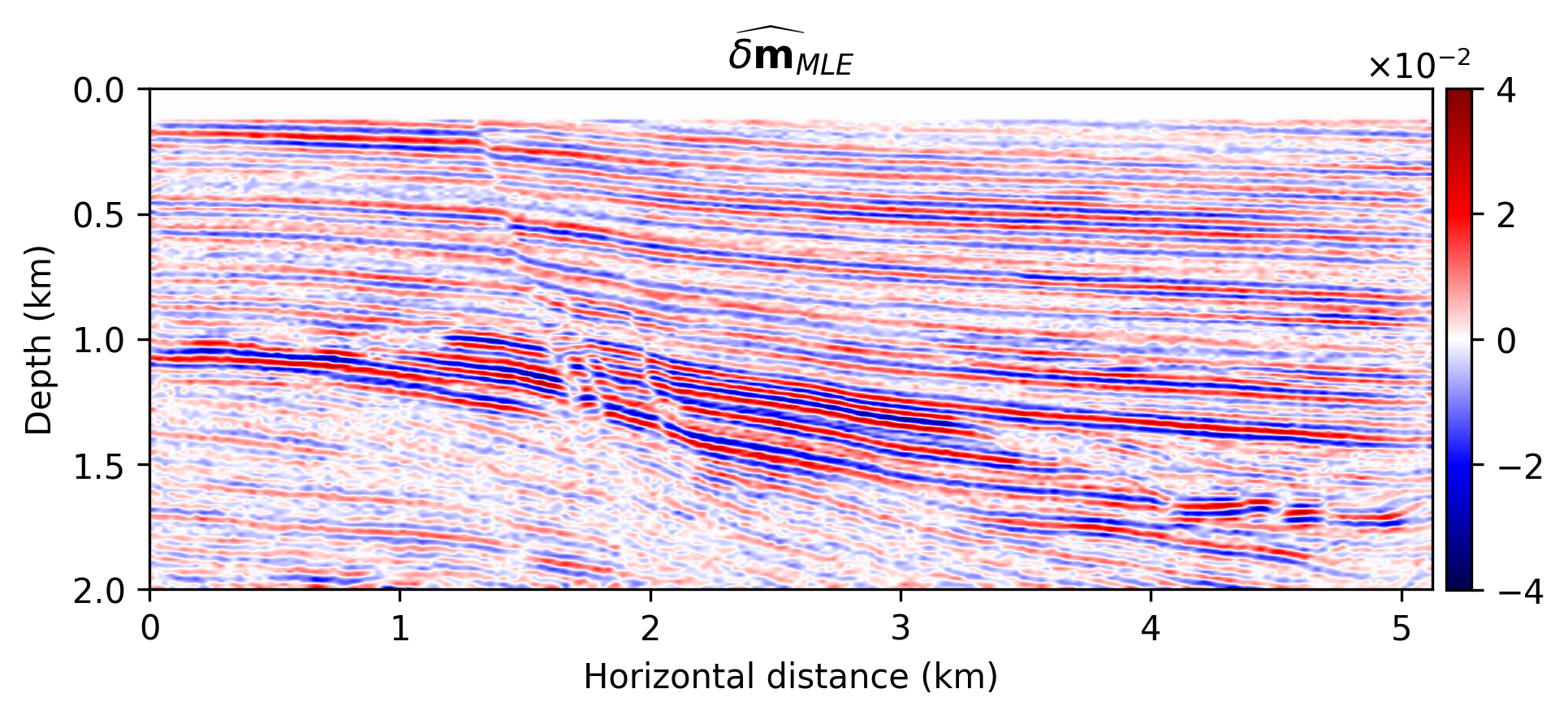
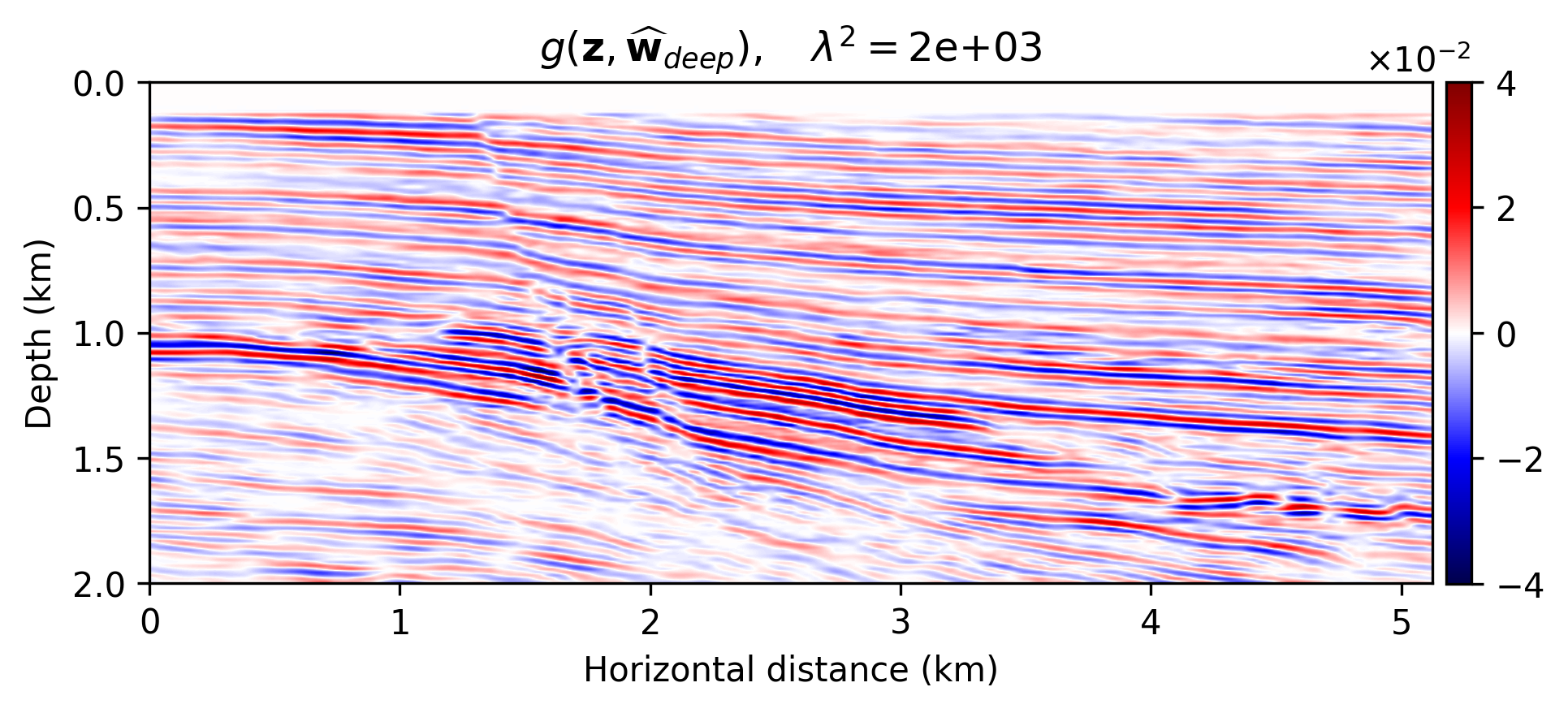
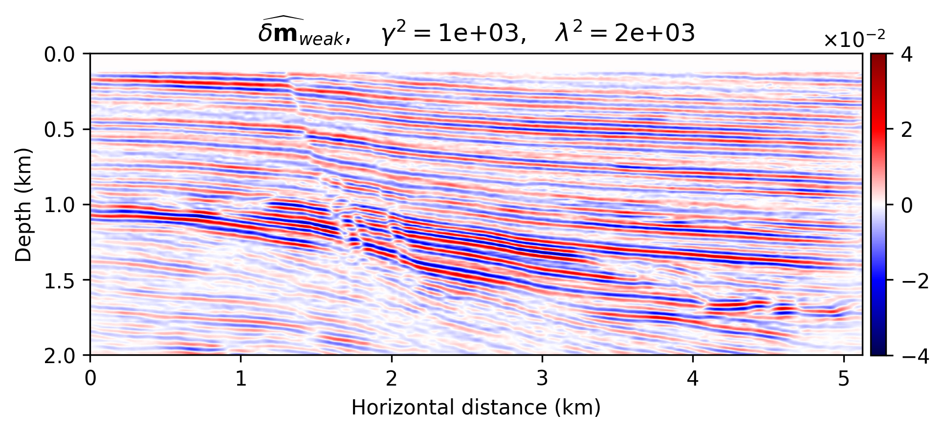
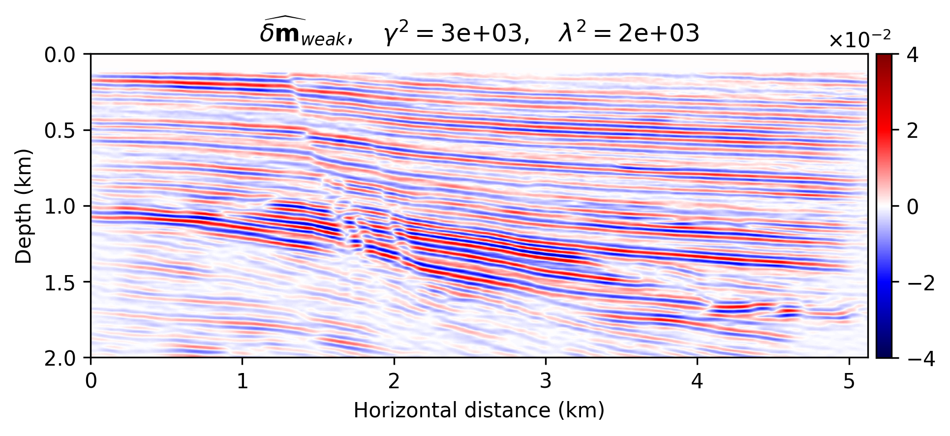
The imaging results are included in Figure 1. Figure 1a indicates the reflectivity that we have used to generate linearized data. Figure 1b is the MLE image—i.e., conventional least-squares reverse-time migration, \(\widehat{\delta \mathbf{m}}_{\text{MLE}}\), obtained by minimizing Equation \(\ref{nll}\) with Adagrad for two passes over the dataset. Figures 1c shows the the deep-prior based image, \(g (\mathbf{z},\widehat{\mathbf{w}}_{\text{deep}})\), computed by running RMSprop for \(15\) passes over the dataset. Figures 1d and 1e show the obtained results using the proposed method by solving problem \(\ref{nlp-weak-deep-prior}\) for two passes over the dataset using values \(\gamma = 10^3\) and \(\gamma = 3 \times 10^3\), respectively.

We make the following observations. As expected, Figure 1b contains imaging artifacts since no prior regularization is in effect. Although the deep prior has been successful in generating a realistic result (Figures \(\ref{nlp-deep-prior}\)), computing the solution required \(15\) passes over the source experiments, which is practically not attainable for larger problems. The solution to the weak deep prior imaging problem, with \(\gamma = 10^3\) (Equation \(\ref{nlp-weak-deep-prior}\)), generates a seismic image with considerably less artifacts compared to MLE (compare Figures 1b and 1d), using the same number of wave-equation solves. By comparing Figure 1d with the image obtained by deep prior based imaging (Figure 1c), we observe that the proposed method is able to provide the benefits of deep prior while remaining computationally feasible. However, Figure 1d is slightly less smooth compared to the true reflectivity (Figure 1a) and deep prior based recovery (Figure 1d). We can increase the the deep prior penalty by increasing \(\gamma\) to \(3 \times 10^3\) (Figure 1e) to get an image with less artifacts compared to Figure 1d. The cost of heavier penalty is amplitude underestimation compared to the deep-prior result (Figure 1c).

Conclusions

The proposed method is an alternative to classical constrained optimization, where handcrafted regularization is considered instead. While practical and ubiquitous, the latter approach is based on heavy-handed assumptions, which inevitably leaves a strong imprint on the final result. Conversely, constraints by deep priors only requires an uninformative Gaussian prior on the network weights. While deep priors have been recently proven successful for many imaging problems, a naive implementation for seismic imaging, which involves lengthy wave-equation solvers, leads to a computationally expensive scheme. By relaxing the deep prior, we decouple model and network updates when optimizing, hence a relatively cheap training phase. As verified by our numerical experiment, we are still able to resolve the imaging artifacts present in conventional least-squares imaging when data is contaminated by strong noise. Compared to reverse-time migration, the deep weak prior approach requires twice its computational cost, an affordable computational budget in large-scale imaging problems.