Abstract
In inverse problems, uncertainty quantification (UQ) deals with a probabilistic description of the solution nonuniqueness and data noise sensitivity. Setting seismic imaging into a Bayesian framework allows for a principled way of studying uncertainty by solving for the model posterior distribution. Imaging, however, typically constitutes only the first stage of a sequential workflow, and UQ becomes even more relevant when applied to subsequent tasks that are highly sensitive to the inversion outcome. In this paper, we focus on how UQ trickles down to horizon tracking for the determination of stratigraphic models and investigate its sensitivity with respect to the imaging result. As such, the main contribution of this work consists in a data-guided approach to horizon tracking uncertainty analysis. This work is fundamentally based on a special reparameterization of reflectivity, known as “deep prior”. Feasible models are restricted to the output of a convolutional neural network with a fixed input, while weights and biases are Gaussian random variables. Given a deep prior model, the network parameters are sampled from the posterior distribution via a Markov chain Monte Carlo method, from which the conditional mean and point-wise standard deviation of the inferred reflectivities are approximated. For each sample of the posterior distribution, a reflectivity is generated, and the horizons are tracked automatically. In this way, uncertainty on model parameters naturally translates to horizon tracking. As part of the validation for the proposed approach, we verified that the estimated confidence intervals for the horizon tracking coincide with geologically complex regions, such as faults.
Introduction
Aside from well data, seismic images are used to delineate stratigraphy. Automatic tracking of the horizons from seismic images (X. Wu and Fomel, 2018; Peters et al., 2019) is becoming a more broadly adapted technology to determine the stratigraphy. While this is a beneficial development, questions remain on its reliability. Even though it is clear that the accuracy of horizon tracking is directly linked to the quality of the seismic image, principled investigations on the risks associated with identifying these horizons are often lacking. Clearly, failure to include uncertainty on tracked horizons may have major implications on the identifications of risks. For this purpose, we propose a technique where we directly translate uncertainty in the image to uncertainty in the tracked horizons. We do this by drawing samples from the posterior distribution of the image followed by automatic horizon tracking. We gain access to samples from the posterior by casting seismic imaging as a Bayesian inversion problem, regularized with a convolutional neural network (CNN), and running preconditioned stochastic gradient Langevin dynamics (pSGLD, Li et al., 2016; Welling and Teh, 2011), a Markov chain Monte Carlo (MCMC) sampler. pSGLD generates an ensemble of reflectivity models, each of which are likely solutions to the imaging problem. Aside from providing information on the point-wise standard deviation of the reflectivity, we use these samples to calculate confidence intervals for our automatically tracked seismic horizons. Compared to conventional imaging and manual tracking of horizons, our combined approach of generating samples from the image posterior and automatic horizon tracking allows us to assess risk in a systematic manner.
While some progress has been made in Uncertainty Quantification (UQ) for seismic imaging (Malinverno, 2002; Malinverno and Briggs, 2004; Malinverno and Parker, 2006; Martin et al., 2012; Ely et al., 2018; Z. Fang et al., 2018; Zhu and Gibson, 2018; Izzatullah et al., 2019; Visser et al., 2019; Zhao and Sen, 2019), further advances are hampered by computational challenges and by over simplifying and often biasing assumptions on parameterizations of the prior and posterior distributions. Motivated by recent developments in machine learning and geophysics (Lempitsky et al., 2018; Cheng et al., 2019; Gadelha et al., 2019; Liu et al., 2019; Y. Wu and McMechan, 2019; Shi et al., 2020; Siahkoohi et al., 2020), we overcome these challenges by parameterizing the unknown reflectivity model in terms of a randomly initialized CNN, where its weights are Gaussian random variables, and sampling the the posterior. Siahkoohi et al. (2020) showed that CNNs act as a regularizer because CNNs tend to generate naturally looking images as long as we prevent them from overfitting. Contrary to early work on deep prior where the optimization is stopped early to prevent overfitting, Siahkoohi et al. (2020) demonstrated that pSGLD avoids fitting the noise and provides samples from the posterior. Through these samples, we are not limited to the maximum a posteriori estimator (MAP), and we are able to compute the conditional mean (known to be relatively more robust with respect to noise artifacts than MAP estimations), and point-wise standard deviation of the image. We track the horizons automatically for each sample of the posterior for the image. This allows us to add confidence intervals to the tracked horizons, which now reflect uncertainties in the image. While we use a deterministic automatic horizon tracking approach (X. Wu and Fomel, 2018), our method will be able to accommodate stochastic horizon tracking schemes—e.g., horizons tracked by many interpretors (Schaaf and Bond, 2019) or by different event tracking softwares.
There have been numerous efforts to incorporate ideas from deep learning in seismic processing and inversion (Ovcharenko et al., 2019; Rizzuti et al., 2019; Siahkoohi et al., 2019a, 2019b, 2019c; Z. Zhang and Alkhalifah, 2019) but there have been relatively few attempts towards UQ. Mosser et al. (2019) use a pretrained generative CNN as a prior in seismic waveform inversion and sample the posterior by running a variant of stochastic gradient Langevin dynamics (SGLD, Welling and Teh, 2011) on the latent variable of the generative CNN. To handle situations where there is no access to training pairs, Herrmann et al. (2019) introduces a formulation that combines handcrafted priors with deep priors to jointly solve the inverse problem and train a model capable of directly sampling the posterior. In this work, we also aim to come up with an unsupervised approach to UQ, but now take it a step further to include a principled way to assess the risk of conducting an additional task on the image, namely tracking the reflector horizons. To our knowledge, our approach is close to recent work by Adler et al. (2018), who proposed a Bayesian framework for jointly performing inversions and tasks. However, our approach differs because it explicitly uses samples from the posterior on the images, by tying uncertainties in the imaging to uncertainties during the subsequent task of of horizon tracking. Our approach also differs fundamentally from other recently developed automatic seismic horizon trackers based on machine learning (see e.g. Peters et al., 2019) because horizon uncertainty is ultimately driven by data (through the intermediate imaging distribution), and not from label (control point) uncertainty.
Our work is organized as follows. We first mathematically formulate how to sample from the image’s posterior distribution by introducing the likelihood function and prior distribution involving the deep prior. Next, we present our approach to quantify the uncertainty in horizon tracking, using samples from the posterior distribution for the image using pSGLD. We conclude by showcasing our approach on synthetic example derived from a 2D portion of a real migrated image of the Parihaka-3D dataset (Veritas, 2005; WesternGeco., 2012), which is used to evaluate automatic horizon tracking algorithms.
Bayesian Seismic Imaging
The objective of seismic imaging is to estimate the reflectivity model, denoted by \(\delta \mathbf{m}\), given observed data, \(\delta \mathbf{d}_{i}\), a smooth background squared-slowness model, \(\mathbf{m}_0\), and assumed to be known seismic source signatures, \(\mathbf{q}_i\), where \(i = 1,2, \cdots , N\) and \(N\) is the number of shot records. To formulate a posterior distribution, in addition to a prior distribution on the reflectivity, we need to specify a likelihood function, \(p_{\text{like}}\) (Tarantola, 2005). Assuming zero-mean Gaussian noise, the negative log-likelihood of the observed data (\(\{\delta \mathbf{d}_i\}_{i=1}^{N}\)) can be written as follows: \[ \begin{equation} \begin{aligned} &\ - \log p_{\text{like}} \left ( \left \{ \delta \mathbf{d}_{i}\right \}_{i=1}^N \normalsize{|} \delta \mathbf{m} \right ) = -\sum_{i=1}^N \log p_{\text{like}} \left ( \delta \mathbf{d}_{i}\normalsize{|} \delta \mathbf{m} \right ) \\ &\ = \frac{1}{2 \sigma^2} \sum_{i=1}^N \| \delta \mathbf{d}_i- \mathbf{J}(\mathbf{m}_0, \mathbf{q}_i) \delta \mathbf{m}\|_2^2 \quad + \underbrace {\text{const}}_{\text{Ind. of } \delta \mathbf{m}}. \\ \end{aligned} \label{imaging-likelihood} \end{equation} \] In this equation, \(\sigma^2\) is the variance of noise in the data and \(\mathbf{J}\) the linearized Born scattering operator computed for a known smooth background model (\(\mathbf{m}_0\)) and source signatures.
Because of noisy data and a nullspace of the Born scattering operator, maximization of the likelihood does not lead to acceptable images and we need to add prior information on the image as a regularization. While many choices for selecting prior distributions exist, they tend to bias MAP or other estimates. We circumvent this bias by using randomly initialized CNNs as priors for the reflectivity model, an approach recently advocated in the literature (Lempitsky et al., 2018; Cheng et al., 2019; Gadelha et al., 2019; Liu et al., 2019; Y. Wu and McMechan, 2019; Shi et al., 2020; Siahkoohi et al., 2020). To this end, we reparameterize the unknown reflectivity model by a randomly initialized CNN—i.e., \(\delta \mathbf{m} = g(\mathbf{z}, \mathbf{w})\), where the vector \(\mathbf{z} \sim \mathrm{N}( \mathbf{0}, \mathbf{I})\) is the fixed input to the CNN. The vector \(\mathbf{w}\) represents the unknown CNN weights. In this formulation, the prior is made of a combination of the functional form of the CNN and a Gaussian prior on the weights—i.e., \(\mathbf{w} \sim \mathrm{N}(\mathbf{0}, \frac{1}{\lambda^2}\mathbf{I})\), where \(\lambda\) is a hyperparameter. Based on these definitions, the negative log-posterior becomes \[ \begin{equation} \begin{aligned} &\ - \log p_{\text{post}} \left ( \mathbf{w} \normalsize{|} \left \{ \delta \mathbf{d}_{i}\right \}_{i=1}^N \right ) \\ &\ = - \left [ \sum_{i=1}^{N} \log p_{\text{like}} \left ( \delta \mathbf{d}_{i}\normalsize{|}\mathbf{w} \right ) \right ] - \log p_{\text{prior}} \left ( \mathbf{w} \right ) + \underbrace {\text{const}}_{\text{Ind. of } \mathbf{w}} \\ &\ = \frac{1}{2 \sigma^2} \sum_{i=1}^N \| \delta \mathbf{d}_i- \mathbf{J}(\mathbf{m}_0, \mathbf{q}_i) {g} (\mathbf{z}, \mathbf{w}) \|_2^2 + \frac{\lambda^2}{2} \| \mathbf{w} \|_2^2 + \text{const,} \\ \end{aligned} \label{imaging-obj} \end{equation} \] where \(p_{\text{post}}\) and \(p_{\text{prior}}\) are the posterior and prior distributions, respectively. In the next section, we present how to draw samples from this posterior distribution.
UQ for Seismic Imaging
MCMC sampling is a well established method to draw samples from unnormalized probability density functions, which in principle makes a suitable candidate for sampling the posterior defined in Equation \(\ref{imaging-obj}\). Unfortunately, MCMC methods become computationally expensive for high-dimensional problems (Z. Fang et al., 2018; Izzatullah et al., 2019; Zhao and Sen, 2019). We employ several strategies to mitigate the costs. For instance, we work with few shot gather stacks randomly formed at each iteration. Secondly, we use a preconditioned version of SGLD proposed by Li et al. (2016). After inclusion of the adaptive diagonal preconditioning matrix \(\mathbf{M}_k\) at the \(k^{\text{th}}\) iteration (see Li et al. (2016) for for detail) the pSGLD update reads \[ \begin{equation} \begin{aligned} &\ \mathbf{w}_{k+1} = \mathbf{w}_{k} - \frac{\epsilon}{2} \mathbf{M}_{k} \nabla_{\mathbf{w}} L^{(i)}(\mathbf{w}_{k}) + \boldsymbol{\eta}_k, \quad \boldsymbol{\eta}_k \sim \mathrm{N}( \mathbf{0}, \epsilon \mathbf{M}_{k}), \\ \end{aligned} \label{sgld} \end{equation} \] where \(L^{(i)} (\mathbf{w}) = \frac{N}{2 \sigma^2} \| \delta \mathbf{d}_i- \mathbf{J}(\mathbf{m}_0, \mathbf{q}_i) {g} (\mathbf{z}, \mathbf{w}) \|_2^2 + \frac{\lambda^2}{2} \| \mathbf{w} \|_2^2\). In this expression, we evaluate the likelihood in Equation \(\ref{imaging-obj}\) by only using the randomly selected \(i^{\text{th}}\) term in the sum. The parameter \(\epsilon\) is the step size. Under certain technical conditions, including properly decaying step sizes, and after an initial “burn-in” phase, the above iterates correspond to samples from the posterior distribution (Li et al., 2016). With these samples, we can approximate expectations, such as the conditional mean, via a sample average over \(T\) realizations—i.e., we have \[ \begin{equation} \begin{aligned} \widehat { \delta \mathbf{m}} &\ = \mathbb{E}_{\mathbf{w} \sim p_{\text{post}} ( \mathbf{w} \normalsize{|} \left \{ \delta \mathbf{d}_{i}\right \}_{i=1}^N )} \left [{g}( \mathbf{z}, \mathbf{w}) \right ] \simeq \frac{1}{T}\sum_{j=1}^{T} {g} \left ( \mathbf{z}, \widehat{\mathbf{w}}_j \right ), \\ \end{aligned} \label{integration} \end{equation} \] where \(\widehat{\mathbf{w}}_j \sim p_{\text{post}} ( \mathbf{w} \normalsize{|} \left \{ \delta \mathbf{d}_{i}\right \}_{i=1}^N ), \ j=1, \ldots, T\). In a similar fashion, point-wise standard deviation can be computed and since it quantifies variability amongst the samples, it contains useful UQ information.
Seismic horizon tracking with UQ
While having access to UQ information in the form of estimated point-wise standard deviation can be useful, one is often more interested in how these uncertainties derived from the data propagate into risks associated with certain tasks conducted on the image. For this purpose, we consider deterministic seismic horizon tracking, which we denote by the mapping \(\mathcal{H}\). Conceptually, this nonlinear mapping represents deterministic actions of automatic horizon trackers or of reliable, consistent human interpreters. In both cases, horizon tracking is not informed by the data other than that is provided with a migrated image. Without loss in generality, we use the automated horizon tracking approach introduced by X. Wu and Fomel (2018), which uses local slopes of the imaged reflectivity to track horizons seeded by user specified control points.
To compute uncertainties on the tracked horizons, we pass the obtained samples from the posterior distribution for the image to the automatic horizon tracking software. Next, by Monte-Carlo integration, we approximate the first and (point-wise) second moment of the posterior distribution for the horizons. The deterministic automatic horizon tracking can be replaced by a nondeterministic approach, reflecting stochasticity in the horizon tracking. Contrary to most existing automatic horizon trackers, the uncertainty in the tracked horizons presented here is due to noise in the shot records and not due uncertainties in the control points as is more commonly studied (see e.g. Peters et al., 2019).
Implementation
The gradient computations required by Equation \(\ref{sgld}\) involve actions of the linearized Born scattering operator and its adjoint and the gradient of the CNN with respect to its weights. For maximal performance, we use Devito (Luporini et al., 2018; M. Louboutin et al., 2019) for the wave-equation based simulations and we integrate matrix-free implementation of these operators into PyTorch (Paszke et al., 2019). In this way, we are able to compute the gradients required in Equation \(\ref{sgld}\) with automatic differentiation. For the CNN architecture, we follow Lempitsky et al. (2018). We use the automated horizon tracking software introduced by X. Wu and Fomel (2018). For more details on our implementation, please refer to our code on GitHub.
Numerical experiments
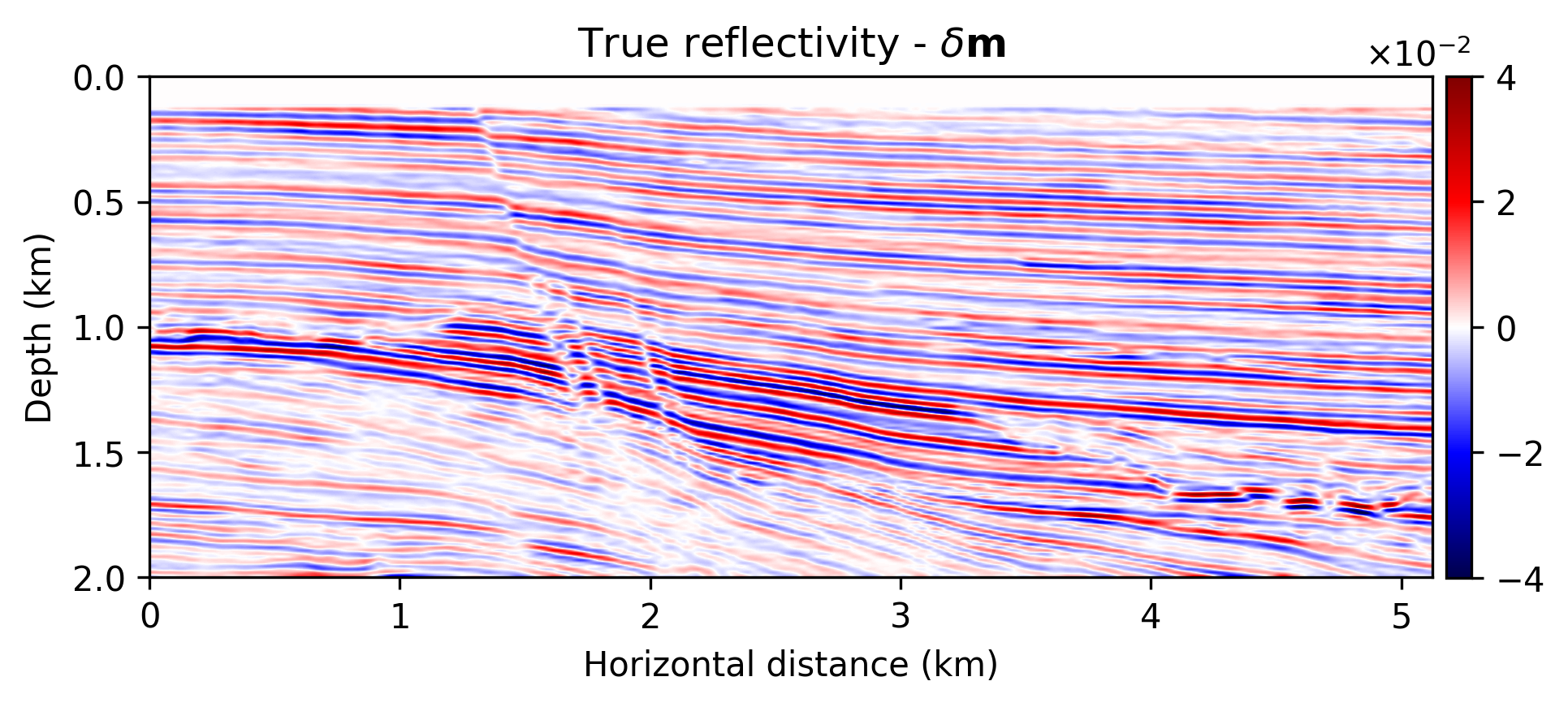
To demonstrate the performance of our approach, we consider a “quasi” real field data example that derives from a 2D subset of the real Kirchoff time migrated Parihaka-3D dataset released by the New Zealand government and used to test the seismic horizon tracker developed by X. Wu and Fomel (2018). We call our experiment quasi real because we generate synthetic data from this “true” imaged reflectivity (see Figure 1a) using our linearized Born scattering operator for a made up, but realistic, smoothly varying background model \(\mathbf{m}_0\). To ensure good coverage, we simulate \(205\) shot records sampled with a source spacing of \(25\, \mathrm{m}\). Each shot is recorded over \(1.5\) seconds with \(410\) fixed receivers sampled at \(12.5 \mathrm{m}\) spread across survey area. The source is a Ricker wavelet with a central frequency of \(30\,\mathrm{Hz}\). To mimic a more realistic imaging scenario, we add a significant amount of noise to the shot records, yielding a low signal-to-noise ratio of the “observed” data of \(-18.01\, \mathrm{dB}\). To limit the computational costs (= number of wave-equation solves), we work with a single simultaneous source, made of a Gaussian weighted source aggregate, per gradient calculation in Equation \(\ref{sgld}\). After an initial burn in of \(3\mathrm{k}\) iterations (about \(15\) passes over the data), we sample every \(20^{\text{th}}\) iteration of the pSGLD iterations in Equation \(\ref{sgld}\). After extensive parameter testing, we set the step size \(\epsilon=0.002\) and penalty parameter \(\lambda^2=200\). The \(\sigma^2=0.01\) equals the variance of the noise we added to the shot records.
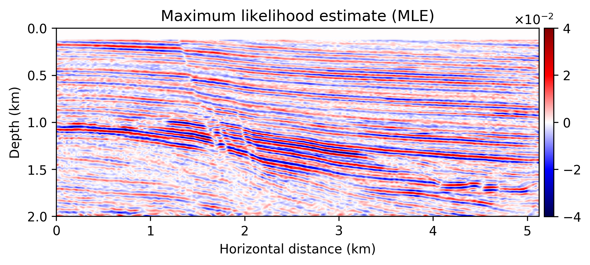
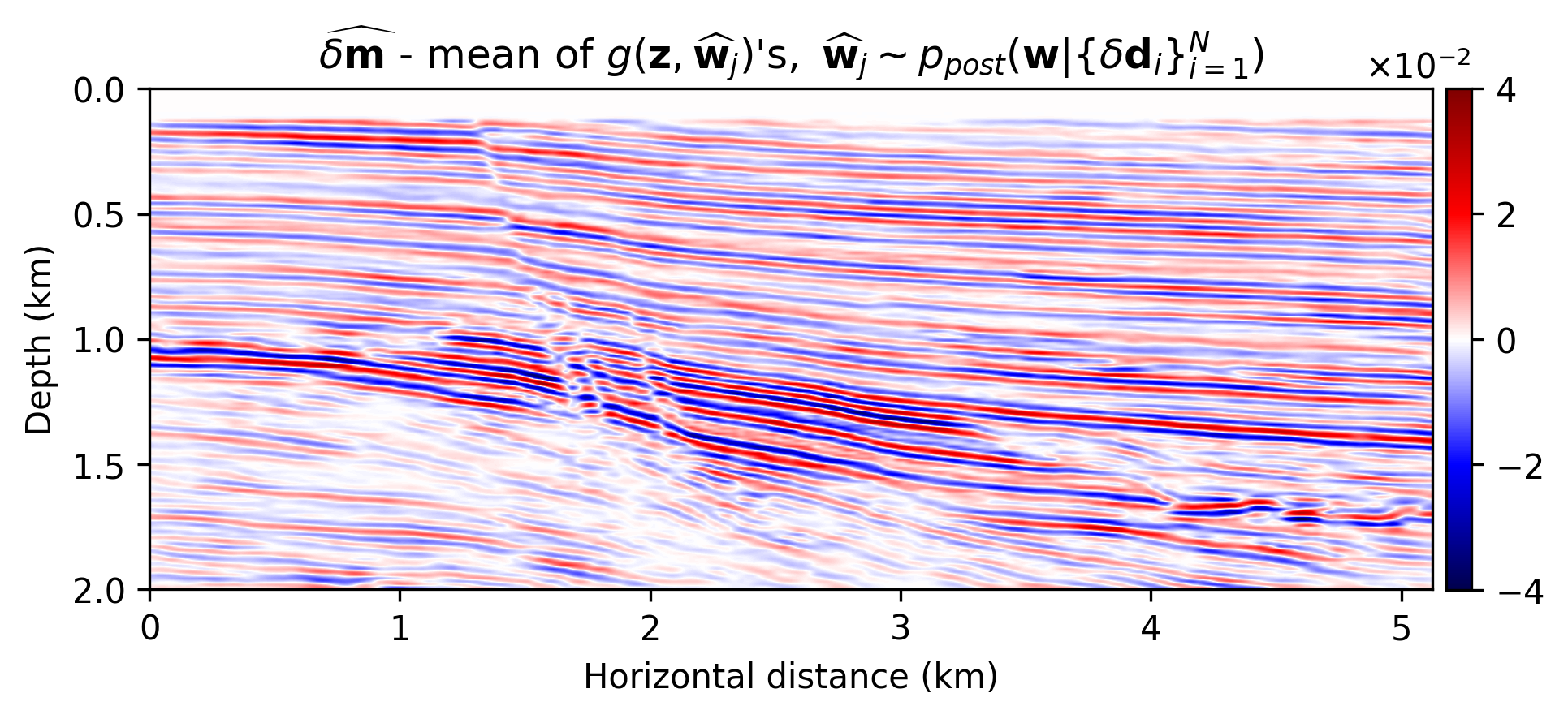
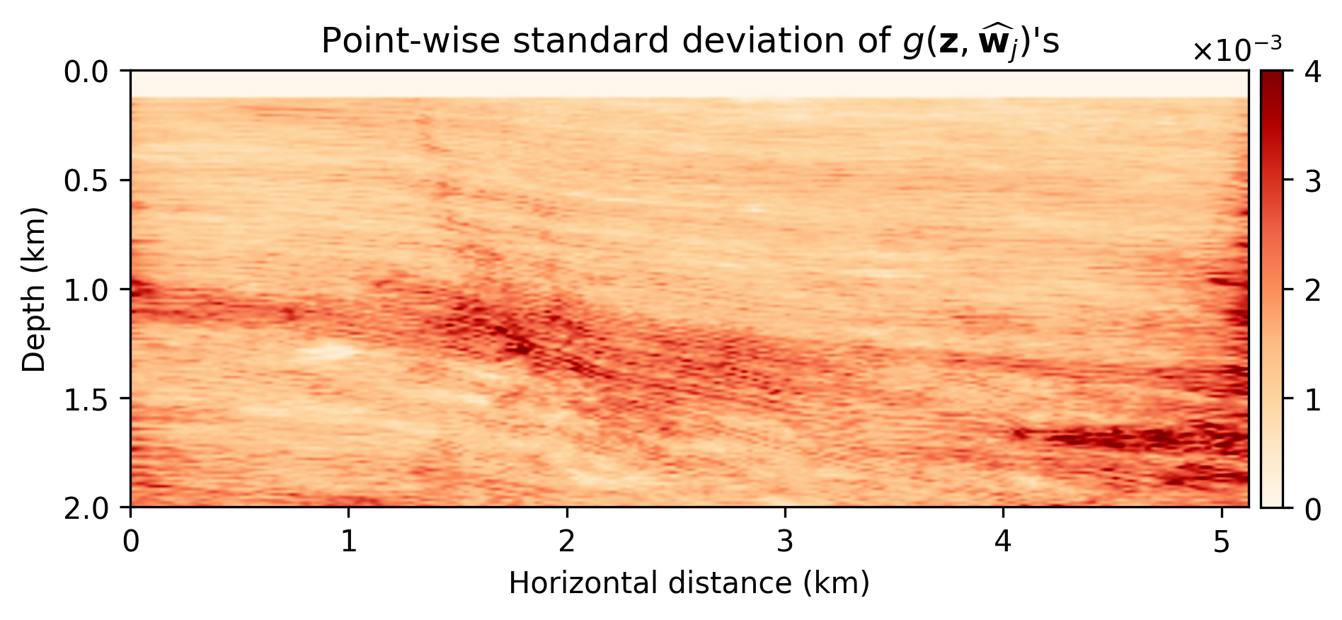
After running \(10\mathrm{k}\) iterations (about \(49\) passes through the data), we sampled \(T=351\) realizations from the posterior distribution on the image. To demonstrate the effect of regularization with the deep prior, we first compute the maximum-likelihood estimate by minimizing Equation \(\ref{imaging-likelihood}\). To avoid overfitting we stop early. The result of this exercise is included in Figure 1b. As expected this result is noisy and above all lacks crucial details and continuity. The estimate for the conditional mean, \(\widehat{\delta \mathbf{m}}\), on the other hand, is much improved, clean and, contains many of the details present in the original “true” reflectivity (cf. Figures 1a – 1c). However, the samples of the posterior do show considerable (up to 10%) variability, as observed in Figure 1d, where the point-wise standard deviation is, as expected, large in areas of complex geology (e.g. near faults and tortuous reflectors) and in areas with a relatively poor illumination.
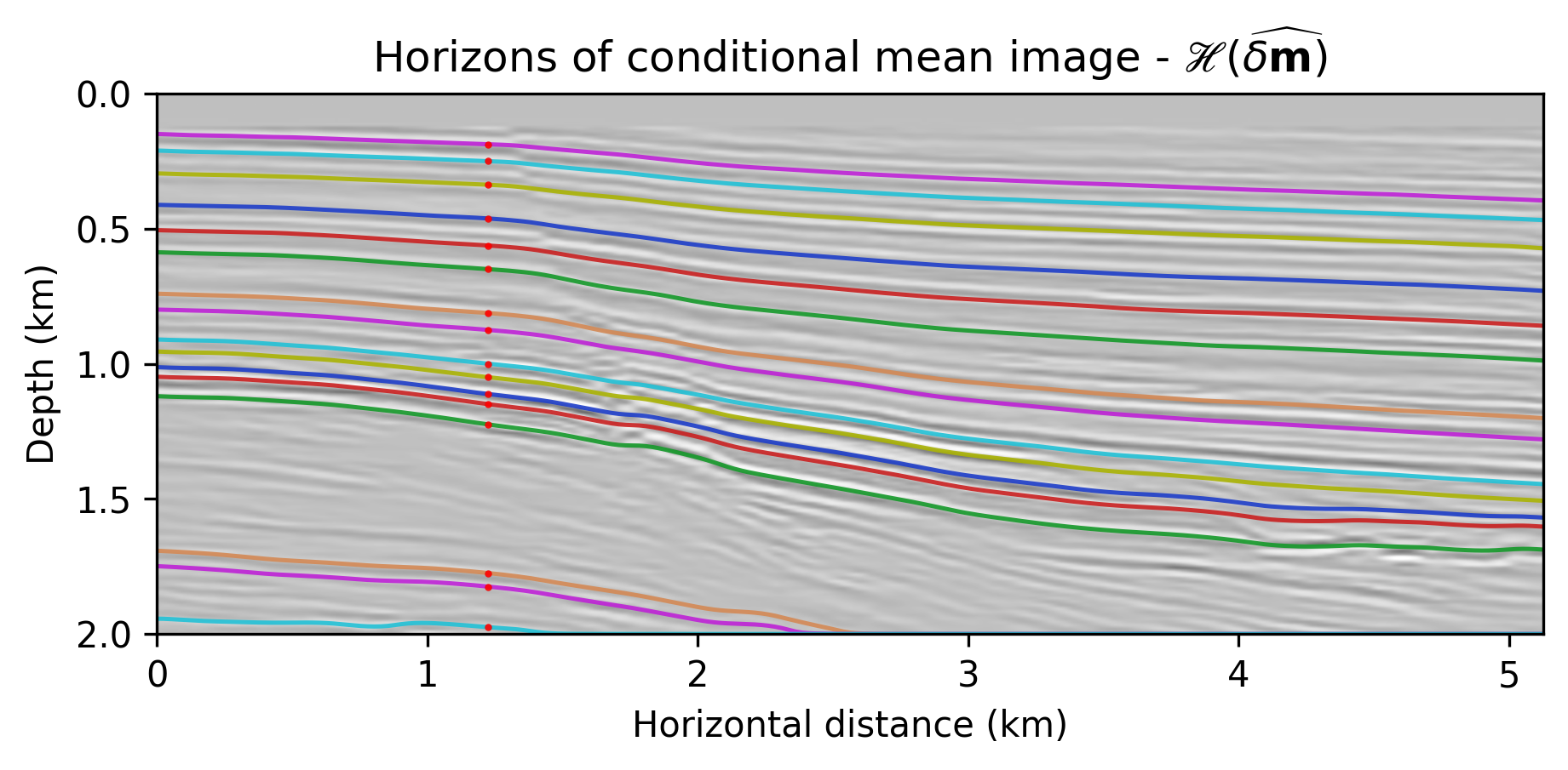
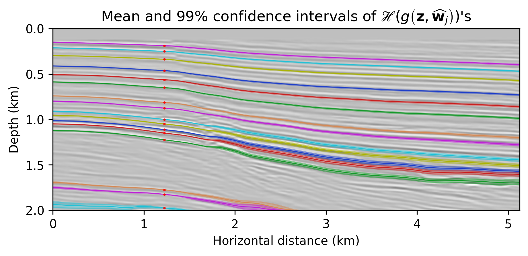
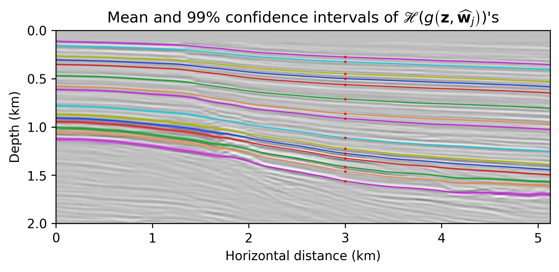
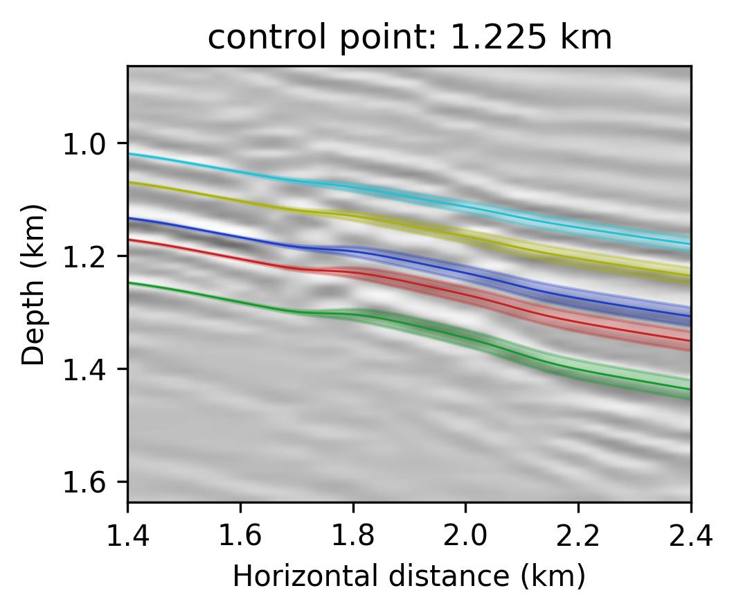
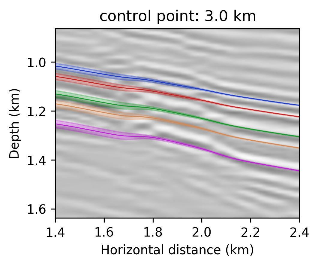
To illustrate how information on the posterior can be used to assess uncertainties in horizon tracking, we use the proposed Monte-Carlo sampling procedure to estimate the conditional mean and the associated \(99\)% confidence interval for a number of reflector horizons. To guide us, we first track horizons on the conditional mean estimate—i.e., \(\mathcal{H}( \widehat{\delta \mathbf{m}})\). We used this estimate to select control points, the red dots located at \(1.225\) \(\mathrm{km}\) horizontal location, that seed the horizon tracker in both directions. While these tracked horizons are close to the conditional mean, \(\mathbb{E}_{\mathbf{w} \sim p_{\text{post}} ( \mathbf{w} \normalsize{|} \left \{ \delta \mathbf{d}_{i} \right \}_{i=1}^N )} \left [ \mathcal{H} \left ( {g}(\mathbf{z},{\mathbf{w}} \right )) \right ]\), their associated confidence intervals in shaded colors exhibit considerable variation. We observe this behavior for different locations of the control points (cf. Figures 2b and 2c) and as we move across faults, areas tortuous reflectivity and into areas of lessened illumination near the edges and in the deeper parts of the image. Depending on the location of the control points, the uncertainty, as expected, increases at the opposite side of the fault. This increase in the size of the confidence interval is due the increased variability amongst samples of the posterior in the region of increased complexity near the fault something we clearly observe in the zoomed figures included in Figures 2d and 2e.
Conclusions
Because of the high dimensionality and complexity of seismic imaging problems, uncertainty quantification remains extremely challenging. In this work, we present a solution for 2D problems by parameterizing seismic images in terms of convolutional neural networks (CNNs) and optimization of the network weights via preconditioned stochastic gradient Langevin dynamics. We showed that the functional form of CNNs, combined with a Gaussian prior on its weights, act as a regularizer and partially circumvent imaging artifacts. Access to the posterior distribution allows us to compute conditional mean, point-wise standard deviation, and confidence intervals for automatically tracked reflector horizons. This is accomplished in a sequential fashion, by computing uncertainties on the imaging result via Monte-Carlo sampling first, and then pushing forward those uncertainties on the tracked horizons. Contrary to most existing horizon tracking approaches, our confidence intervals are driven by noise in the shot records and not from control point errors. In this work, control points were calculated from the conditional mean imaging result, but information coming from well logs can be in principle integrated as well. Our approach can further include control point uncertainty, or applied to other tasks, such as image segmentation. This work is, to our knowledge, one of the first instances where data errors—e.g., due to noise or linearization approximations, are systematically mapped to confidence interval of some imaging result attributes.
Acknowledgments
The authors thank Charles Jones for constructive conversations and comments.
Adler, J., Lunz, S., Verdier, O., Schönlieb, C.-B., and Öktem, O., 2018, Task adapted reconstruction for inverse problems: ArXiv Preprint ArXiv:1809.00948.
Cheng, Z., Gadelha, M., Maji, S., and Sheldon, D., 2019, A Bayesian Perspective on the Deep Image Prior: In The IEEE Conference on Computer Vision and Pattern Recognition (CVPR) (pp. 5443–5451).
Ely, G., Malcolm, A., and Poliannikov, O. V., 2018, Assessing uncertainties in velocity models and images with a fast nonlinear uncertainty quantification method: GEOPHYSICS, 83, R63–R75. doi:10.1190/geo2017-0321.1
Fang, Z., Silva, C. D., Kuske, R., and Herrmann, F. J., 2018, Uncertainty quantification for inverse problems with weak partial-differential-equation constraints: GEOPHYSICS, 83, R629–R647. doi:10.1190/geo2017-0824.1
Gadelha, M., Wang, R., and Maji, S., 2019, Shape reconstruction using differentiable projections and deep priors: In Proceedings of the iEEE international conference on computer vision (pp. 22–30).
Herrmann, F. J., Siahkoohi, A., and Rizzuti, G., 2019, Learned imaging with constraints and uncertainty quantification: Neural Information Processing Systems (NeurIPS) 2019 Deep Inverse Workshop. Retrieved from https://arxiv.org/pdf/1909.06473.pdf
Izzatullah, M., Leeuwen, T. van, and Peter, D., 2019, Bayesian uncertainty estimation for full waveform inversion: A numerical study: SEG Technical Program Expanded Abstracts 2019. doi:10.1190/segam2019-3216008.1
Lempitsky, V., Vedaldi, A., and Ulyanov, D., 2018, Deep Image Prior: In 2018 iEEE/CVF conference on computer vision and pattern recognition (pp. 9446–9454). doi:10.1109/CVPR.2018.00984
Li, C., Chen, C., Carlson, D., and Carin, L., 2016, Preconditioned stochastic gradient Langevin dynamics for deep neural networks: In Thirtieth AAAI Conference on Artificial Intelligence.
Liu, Q., Fu, L., and Zhang, M., 2019, Deep-seismic-prior-based reconstruction of seismic data using convolutional neural networks: ArXiv Preprint ArXiv:1911.08784.
Louboutin, M., Lange, M., Luporini, F., Kukreja, N., Witte, P. A., Herrmann, F. J., … Gorman, G. J., 2019, Devito (v3.1.0): An embedded domain-specific language for finite differences and geophysical exploration: Geoscientific Model Development, 12, 1165–1187. doi:10.5194/gmd-12-1165-2019
Luporini, F., Lange, M., Louboutin, M., Kukreja, N., Hückelheim, J., Yount, C., … Gorman, G. J., 2018, Architecture and performance of devito, a system for automated stencil computation: CoRR, abs/1807.03032. Retrieved from http://arxiv.org/abs/1807.03032
Malinverno, A., 2002, Parsimonious bayesian markov chain monte carlo inversion in a nonlinear geophysical problem: Geophysical Journal International, 151, 675–688. doi:10.1046/j.1365-246X.2002.01847.x
Malinverno, A., and Briggs, V. A., 2004, Expanded uncertainty quantification in inverse problems: Hierarchical bayes and empirical bayes: GEOPHYSICS, 69, 1005–1016. doi:10.1190/1.1778243
Malinverno, A., and Parker, R. L., 2006, Two ways to quantify uncertainty in geophysical inverse problems: GEOPHYSICS, 71, W15–W27. doi:10.1190/1.2194516
Martin, J., Wilcox, L. C., Burstedde, C., and Ghattas, O., 2012, A Stochastic Newton MCMC Method for Large-scale Statistical Inverse Problems with Application to Seismic Inversion: SIAM Journal on Scientific Computing, 34, A1460–A1487. Retrieved from http://epubs.siam.org/doi/abs/10.1137/110845598
Mosser, L., Dubrule, O., and Blunt, M., 2019, Stochastic Seismic Waveform Inversion Using Generative Adversarial Networks as a Geological Prior: Mathematical Geosciences, 84, 53–79. doi:10.1007/s11004-019-09832-6
Ovcharenko, O., Kazei, V., Kalita, M., Peter, D., and Alkhalifah, T. A., 2019, Deep learning for low-frequency extrapolation from multi-offset seismic data: GEOPHYSICS, 84, R989–R1001. doi:10.1190/geo2018-0884.1
Paszke, A., Gross, S., Massa, F., Lerer, A., Bradbury, J., Chanan, G., … Chintala, S., 2019, PyTorch: An Imperative Style, High-Performance Deep Learning Library: In Advances in neural information processing systems 32 (pp. 8024–8035). Retrieved from http://papers.neurips.cc/paper/9015-pytorch-an-imperative-style-high-performance-deep-learning-library.pdf
Peters, B., Granek, J., and Haber, E., 2019, Multiresolution neural networks for tracking seismic horizons from few training images: Interpretation, 7, SE201–SE213. doi:10.1190/INT-2018-0225.1
Rizzuti, G., Siahkoohi, A., and Herrmann, F. J., 2019, Learned iterative solvers for the Helmholtz equation: 81st EAGE Conference and Exhibition 2019. doi:10.3997/2214-4609.201901542
Schaaf, A., and Bond, C. E., 2019, Quantification of uncertainty in 3-D seismic interpretation: Implications for deterministic and stochastic geomodeling and machine learning: Solid Earth.
Shi, Y., Wu, X., and Fomel, S., 2020, Deep learning parameterization for geophysical inverse problems: In SEG 2019 Workshop: Mathematical Geophysics: Traditional vs Learning, Beijing, China, 5-7 November 2019 (pp. 36–40). Society of Exploration Geophysicists. doi:10.1190/iwmg2019_09.1
Siahkoohi, A., Kumar, R., and Herrmann, F. J., 2019a, Deep-learning based ocean bottom seismic wavefield recovery: SEG Technical Program Expanded Abstracts 2019. doi:10.1190/segam2019-3216632.1
Siahkoohi, A., Louboutin, M., and Herrmann, F. J., 2019b, The importance of transfer learning in seismic modeling and imaging: GEOPHYSICS, 84, A47–A52. doi:10.1190/geo2019-0056.1
Siahkoohi, A., Rizzuti, G., and Herrmann, F. J., 2020, A deep-learning based bayesian approach to seismic imaging and uncertainty quantification: 82nd EAGE Conference and Exhibition 2020. Retrieved from https://slim.gatech.edu/Publications/Public/Submitted/2020/siahkoohi2020EAGEdlb/siahkoohi2020EAGEdlb.html
Siahkoohi, A., Verschuur, D. J., and Herrmann, F. J., 2019c, Surface-related multiple elimination with deep learning: SEG Technical Program Expanded Abstracts 2019. doi:10.1190/segam2019-3216723.1
Tarantola, A., 2005, Inverse problem theory and methods for model parameter estimation: SIAM. doi:10.1137/1.9780898717921
Veritas, 2005, Parihaka 3D Marine Seismic Survey - Acquisition and Processing Report: No. New Zealand Petroleum Report 3460. New Zealand Petroleum & Minerals, Wellington.
Visser, G., Guo, P., and Saygin, E., 2019, Bayesian transdimensional seismic full-waveform inversion with a dipping layer parameterization: GEOPHYSICS, 84, R845–R858. doi:10.1190/geo2018-0785.1
Welling, M., and Teh, Y. W., 2011, Bayesian Learning via Stochastic Gradient Langevin Dynamics: In Proceedings of the 28th International Conference on International Conference on Machine Learning (pp. 681–688).
WesternGeco., 2012, Parihaka 3D PSTM Final Processing Report: No. New Zealand Petroleum Report 4582. New Zealand Petroleum & Minerals, Wellington.
Wu, X., and Fomel, S., 2018, Least-squares horizons with local slopes and multi-grid correlations: GEOPHYSICS, 83, IM29–IM40. doi:10.1190/geo2017-0830.1
Wu, Y., and McMechan, G. A., 2019, Parametric convolutional neural network-domain full-waveform inversion: GEOPHYSICS, 84, R881–R896. doi:10.1190/geo2018-0224.1
Zhang, Z., and Alkhalifah, T., 2019, Regularized elastic full waveform inversion using deep learning: GEOPHYSICS, 84, 1SO–Z28. doi:10.1190/geo2018-0685.1
Zhao, Z., and Sen, M. K., 2019, A gradient based MCMC method for FWI and uncertainty analysis: SEG Technical Program Expanded Abstracts 2019. doi:10.1190/segam2019-3216560.1
Zhu, D., and Gibson, R., 2018, Seismic inversion and uncertainty quantification using transdimensional markov chain monte carlo method: GEOPHYSICS, 83, R321–R334. doi:10.1190/geo2016-0594.1