Parameterizing uncertainty by deep invertible networks, an application to reservoir characterization

Abstract

Uncertainty quantification for full-waveform inversion provides a probabilistic characterization of the ill-conditioning of the problem, comprising the sensitivity of the solution with respect to the starting model and data noise. This analysis allows to assess the confidence in the candidate solution and how it is reflected in the tasks that are typically performed after imaging (e.g., stratigraphic segmentation following reservoir characterization). Classically, uncertainty comes in the form of a probability distribution formulated from Bayesian principles, from which we seek to obtain samples. A popular solution involves Monte Carlo sampling. Here, we propose instead an approach characterized by training a deep network that “pushes forward” Gaussian random inputs into the model space (representing, for example, density or velocity) as if they were sampled from the actual posterior distribution. Such network is designed to solve a variational optimization problem based on the Kullback-Leibler divergence between the posterior and the network output distributions. This work is fundamentally rooted in recent developments for invertible networks. Special invertible architectures, besides being computational advantageous with respect to traditional networks, do also enable analytic computation of the output density function. Therefore, after training, these networks can be readily used as a new prior for a related inversion problem. This stands in stark contrast with Monte-Carlo methods, which only produce samples. We validate these ideas with an application to angle-versus-ray parameter analysis for reservoir characterization.

Introduction

A classical probabilistic setup for full-waveform inversion (FWI, Tarantola, 2005) starts from the following assumptions on the data likelihood: \[ \begin{equation} \bd=\F(\bm)+\bn. \label{eq_like} \end{equation} \] Here, \(\bd\) represents seismic data, \(\F\) is the forward modeling map, \(\bm\) collects the unknown medium parameters of interest, and \(\bn\) is random noise. We are assuming that \(\bd\) and \(\bn\) are independent (knowing \(\bm\)), and \(\bn\sim\pnoise(\bn)\) is normally distributed according to \(\Normal(0,I)\). Equation \(\eqref{eq_like}\) then defines the likelihood density function \[ \begin{equation*} \bd|\bm\sim\like(\bd|\bm)=\pnoise(\bd-\F(\bm)). \end{equation*} \] In the Bayesian framework, the second ingredient is a prior distribution on the model space \[ \begin{equation} \bm\sim\prior(\bm). \label{eq_prior} \end{equation} \] Since for seismic experiments we do not have direct access to the Earth’s interior (except for localized information in the form of well logs), the prior is typically hand crafted based on, e.g., Thikhonov or total variation regularization (see, for example, Esser et al., 2018; Peters et al., 2019). Alternatively, when this type of information is available, a prior can be implicitly encoded via a deep network (Mosser et al., 2019).

The posterior distribution, given data \(\bd\), is readily obtained from the Bayes’ rule: \[ \begin{equation} \post(\bm|\bd)=\like(\bd|\bm)\prior(\bm)/\pdata(\bd), \label{eq_post} \end{equation} \] where \(\pdata(\bd)=\int\like(\bd|\bm)\prior(\bm)\,\mathrm{d}\bm\). Sampling from the posterior probability \(\eqref{eq_post}\) is the goal of uncertainty quantification (UQ). Besides the usual maximum-a-posteriori estimator (MAP) \[ \begin{equation} \bm_{\mathrm{MAP}}=\arg\max_{\bm}\post(\bm|\bd), \label{eq_map} \end{equation} \] being able to sample from the posterior allows to approximate the conditional mean and point-wise standard deviation: \[ \begin{equation} \begin{aligned} & \mu = \E(\bm|\bd)=\int\bm\,\post(\bm|\bd)\,\mathrm{d}\bm,\\ & \sigma^2 = \E((\bm-\mu)^{.2}|\bd)=\int(\bm-\mu)^{.2}\post(\bm|\bd)\,\mathrm{d}\bm. \end{aligned} \label{eq_condest} \end{equation} \] A great deal of research around UQ is devoted to Monte Carlo sampling (Robert and Casella, 2004), especially through Markov chains (MCMC) when dealing with high-dimensional problems like FWI (see, e.g., Malinverno and Briggs, 2004; Bennett and Malinverno, 2005; Malinverno and Parker, 2006; Martin et al., 2012; Sambridge et al., 2013; Ely et al., 2018; Parno and Marzouk, 2018; D. Zhu and Gibson, 2018; Izzatullah et al., 2019; Visser et al., 2019; Zhao and Sen, 2019). A Markov chain is a stochastic process that describes the evolution of the model distribution, and is designed to match the target distribution at steady state. A particularly egregious example is offered by the so-called Langevin dynamics (Neal and others, 2011): \[ \begin{equation} \bm_{n+1}=\bm_n-\frac{\varepsilon_n}{2}\nabla_{\bm}\log\post(\cdot|\bd)|_{\bm_n}+\eta_n,\quad\eta_n\sim\Normal(0,\varepsilon_nI), \label{eq_langevin} \end{equation} \] which is akin to stochastic gradient descent where the update direction is perturbed by random noise \(\eta_n\). Under some technical assumptions on the step-length decaying (Welling and Teh, 2011), collecting \(\bm_n\)’s as in Equation \(\eqref{eq_langevin}\) is equivalent to sample from the posterior distribution (after an initial “burn-in” phase). While gradient-based sampling methods such as Langevin dynamics are gaining popularity in machine learning, we must face the computational challenge given by the evaluation and differentiation of the seismic modeling map involved in Equation \(\eqref{eq_langevin}\), which needs be repeated for multiple sources thus resulting in an expensive scheme. Nevertheless, source encoding and network reparameterization could alleviate these issues (Herrmann et al., 2019; Siahkoohi et al., 2020a, 2020b).

In this paper, we take an alternative route to UQ by employing model-space valued deep networks defined on a latent space endowed with an easy-to-sample distribution (e.g. normal), as a way to mimic random sampling from the posterior (when properly trained). This is made possible by a special class of invertible networks for which the output density function can be computed analytically (Dinh et al., 2016; Kingma and Dhariwal, 2018; Lensink et al., 2019; Kruse et al., 2019). As such, these networks encapsulate a new prior, which can be used for subsequent tasks (as, for example, a similar imaging problem).

Method

In this section, we discuss the theoretical foundations of the proposed method for UQ via generative networks. We start by discussing a well-known notion of discrepancy between probabilities, the Kullback-Leibler divergence. Our program is suggested in Kruse et al. (2019), and entails the minimization of the posterior divergence with a known distribution pushed forward by an invertible mapping. The resulting optimization problem is further restricted over a special class of invertible networks, for which the log-determinant of the Jacobian can be computed.

The Kullback-Leibler (KL) divergence of two probabilities defined on the model space \(\bm\in\M\), with density \(p\) and \(q\) respectively, is given by \[ \begin{equation} \KL(p||q)=\int p(\bm)\log\dfrac{p(\bm)}{q(\bm)}\,\mathrm{d}\bm. \label{eq_KL} \end{equation} \] Let us fix, now, a normally distributed random variable \[ \begin{equation} \bz\sim\plat(\bz), \label{eq_Zlat} \end{equation} \] taking values on a latent space \(\Z\), and a deterministic map \[ \begin{equation} \T:\Z\to\M. \label{eq_T} \end{equation} \] Selecting random samples \(\bz\) and feeding it to \(\T\) generates a random variable \(\T(\bz)\) with values in \(\M\), which is referred to as the push-forward of \(\bz\) through \(\T\). The push-forward density will be denoted by \[ \begin{equation} \bm\sim\T_{\#}\plat(\bm). \label{eq_pushfw} \end{equation} \] Our goal is the solution of the following minimization problem: \[ \begin{equation} \min_T\KL(\T_{\#}\plat||\post). \label{eq_KLmin} \end{equation} \] Note that the KL divergence is notoriously not symmetric, and the order of the probabilities appearing in Equation \(\eqref{eq_KLmin}\) is designed. A more convenient form of Equation \(\eqref{eq_KLmin}\) is \[ \begin{equation} \begin{split} \KL(\T_{\#}\plat||\post)=\E_{\bz\sim\plat(\bz)}-\log\post(T(\bz)|\bd)\\-H(\T_{\#}\plat), \end{split} \label{eq_KLminEntr} \end{equation} \] where \[ \begin{equation} H(p)=-\int p(\bm)\log p(\bm)\,\mathrm{d}\bm \label{eq_entropy} \end{equation} \] denotes the entropy of \(p\). The loss function in Equation \(\eqref{eq_KLminEntr}\) ensures that the outputs of \(\T\) adhere to the data without producing mode collapse (e.g. \(T(\bz)\equiv\bm_{\mathrm{MAP}}\), a low-entropy configuration).

While the first term in the KL divergence can be approximated by sample averaging, i.e. \(\E_{\bz\sim\plat(\bz)}f(\bz)\approx\frac{1}{N}\sum_{i=1}^Nf(\bz_i)\), calculating the entropy of a push-forward distribution is not trivial (see, for instance, Kim and Bengio, 2016). In general, we typically can only evaluate \(T(\bz)\) without a direct way to explicitly compute its density, as in Equation \(\eqref{eq_pushfw}\), for a given \(\bm\). A popular—but computationally expensive—workaround is based on generative adversarial networks (GAN, Goodfellow et al., 2014), where the discriminator is in fact related to the generator push-forward density (Che et al., 2020). Other approaches involve variational autoencoders (Kingma and Welling, 2013) and expectation-maximization techniques (Han et al., 2017). Nevertheless, if we focus on the specialized class of invertible mappings \(\T\) (whose existence requires that \(\dim\Z=\dim\M\) as manifolds), we obtain \[ \begin{equation} H(\T_{\#}\plat)=H(\plat)+\E_{\bz\sim\plat(\bz)}\log|\det J_{\T}(\bz)| \label{eq_entropyinv} \end{equation} \] thanks to the change-of-variable formula. Here, \(J_{\T}(\bz)\) is the Jacobian of \(\T\) with respect to the input \(\bz\).

Invertible networks are an enticing family of choice for \(\T\). This is especially true for sizable inverse problems, since they do not require storing the input before every activation functions (such as ReLU) and the memory overhead can be kept constant (Putzky and Welling, 2019). Furthermore, recent developments has lead to architectures that allows the computation (and differentiation) of the log-determinants that appears in Equation \(\eqref{eq_entropyinv}\). As notable examples, we mention non-volume-preserving networks (NVP, Dinh et al., 2016), generative flows with invertible 1-by-1 convolutions (Glow, Kingma and Dhariwal, 2018), and hierarchically invertible neural transport (HINT, Kruse et al., 2019). These examples share the usage of special bijective layers whose Jacobian has a triangular structure (Knothe-Rosenblatt transformations, Parno and Marzouk, 2018). Hyperbolic networks (Lensink et al., 2019) are another instance of invertible maps, although volume preserving with null log-determinants. An invertible version of classical residual networks (resnets) is also offered in Behrmann et al. (2018), which however requires an implicit estimation of the log-determinant. Yet another example of invertible architecture, though not allowing log-determinant calculation, is discussed in Putzky and Welling (2019) for inverse problem applications.

By restricting the problem in Equation \(\eqref{eq_KLmin}\) to the family of suitable invertible networks just described, we end up with the following optimization: \[ \begin{equation} \begin{split} \min_{\theta}\E_{\bz\sim\plat(\bz)}\frac{1}{2}\norm{\bd-\F(G_{\theta}(\bz))}^2-\log\prior(G_{\theta}(\bz))\\-\log|\det J_{G_{\theta}}(\bz)|, \end{split} \label{eq_uqprob} \end{equation} \] where the unknowns \(\theta\) represent the parameters (such as weights and biases) of the invertible network \[ \begin{equation} G_{\theta}:\Z\to\M,\quad G_{\theta}^{-1}:\M\to\Z. \label{eq_invnets} \end{equation} \] We employ a stochastic gradient approach (ADAM, Kingma and Ba, 2014) with random selection of normally distributed mini-batches of \(\bz\)’s. The expectation in Equation \(\eqref{eq_uqprob}\) is then replaced by Monte-Carlo averaging.

The solution of problem \(\eqref{eq_uqprob}\) comes in the form of a network \(G_{\theta}\), whose evaluation over random \(\bz\)’s generates models \(\bm\)’s as if they were sampled from the posterior distribution in Equation \(\eqref{eq_post}\). After training, we can easily compute conditional mean and point-wise standard deviation as in Equation \(\eqref{eq_condest}\), or even higher-order statistics. Since \(G_{\theta}\) possesses a suitable architecture that explicitly encodes its output density, we can reuse this result as a new prior for adiacent regions, time-lapse imaging, and so on.

Uncertainty quantification for reservoir characterization

We now apply the setup described in the previous section, Equation \(\eqref{eq_uqprob}\), to full-waveform inversion for reservoir characterization under some simplifying assumptions. We postulate a purely acoustic model (constant density), with laterally homogeneous properties (e.g., 1D). Waves propagate in a 2D medium. The Radon transform yields the “1.5-D” wave equation \[ \begin{equation} (\bm(z)-p^2)\partial_{tt}\bu(t, z, p)-\partial_{zz}\bu(t, z, p)=\bq(t)\delta(z), \label{eq_waveq} \end{equation} \] where \(\bu\) is a wavefield, \(\bq\) a source wavelet, and \(p\) the ray parameter. Time-depth is indicated by \((t,z)\). Data is collected at the surface \(z=0\).

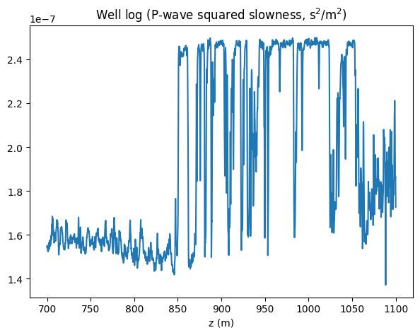
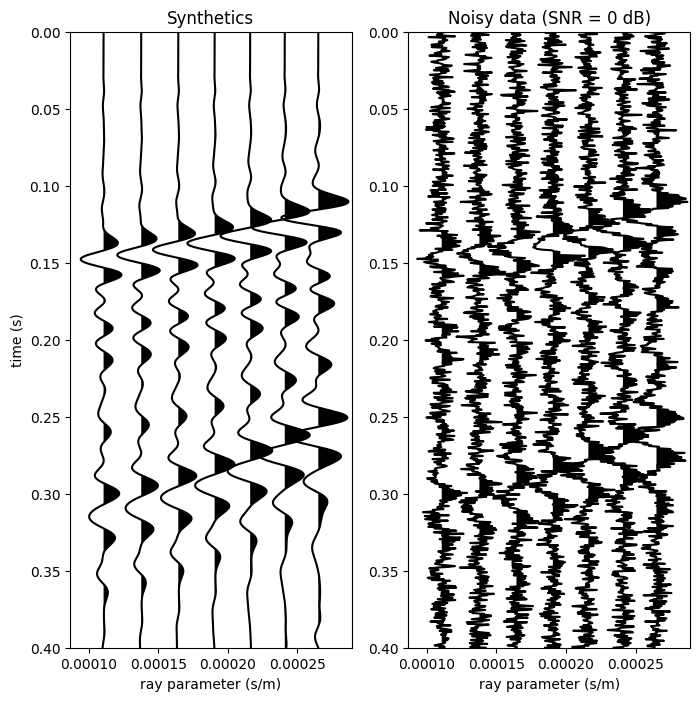
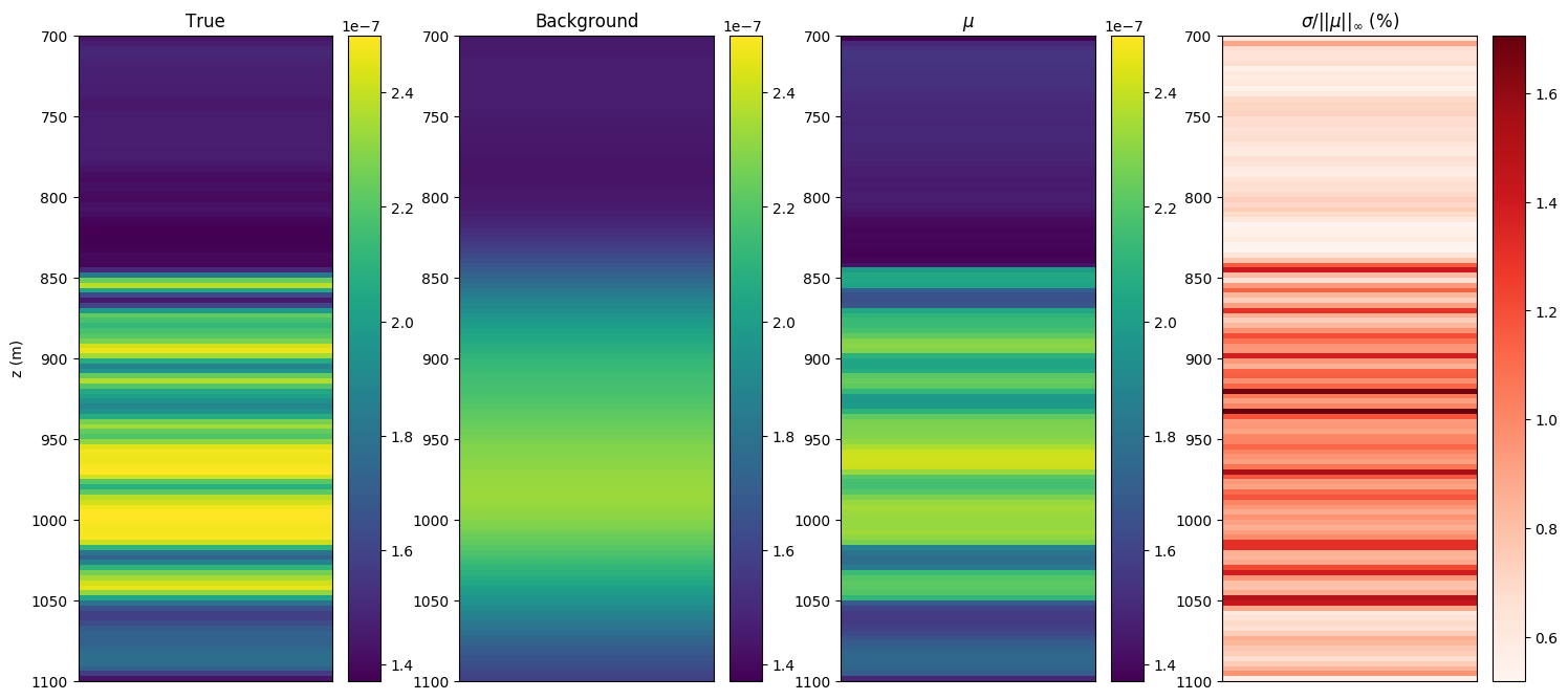
We synthetize a compressional velocity well-log from the open-source Sleipner dataset in Figure 1 (refer to Haffinger et al., 2018 for a previous AVP study). See the acknowledgements for more info. The true model is obtained by smoothing and subsampling the well-log slowness on a \(3\) m grid, and a background is obtained by severe smoothing. We select a source wavelet with corner frequencies \((5, 30, 50, 80)\) Hz, and a angle range from \(\theta=12^{\circ}\) to \(\theta=30^{\circ}\), where \(p=\sin\theta\sqrt{\bm(z=0)}\). Synthetic data are generated by finite-differences, and random Gaussian noise is injected with \(\mathrm{SNR}=0\) dB. Data are shown in Figure 2.

As of invertible architecture, we choose hyperbolic networks (Lensink et al., 2019), due to their inherent stability, augmented with one activation normalization layer (similarly to Kingma and Dhariwal, 2018) acting diagonally along the depth dimension. This modification is necessary to obtain a non-volume preserving transformation, that is with a non-null log-determinant (otherwise the network entropy will remain constant, cf. Equation \(\ref{eq_entropyinv}\)).

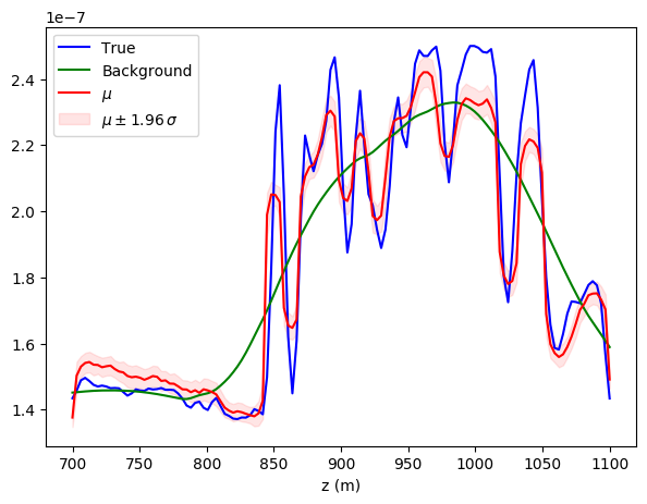
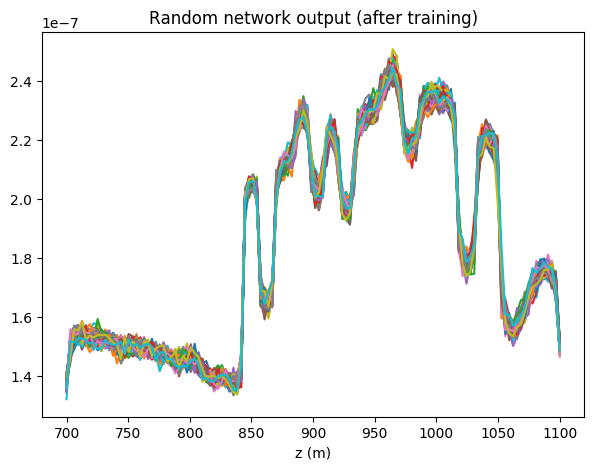
The inversion results are compared in Figure 3. We plot the conditional mean \(\mu\), as defined in Equation \(\eqref{eq_condest}\), with confidence intervals determined by the pointwise conditional standard deviation \(\sigma\). The conditional \(\mu\) and \(\sigma\) are calculated with sample average of the network outputs \(G_{\theta}(\bz)\). Additionally we show multiple samples from the estimated posterior before and after training (Figure 4), which highlight the sharpening of the distribution around the mean once optimized. Note that \(G_{\theta}\) was initialized as Gaussian perturbations of the MAP, cf. Figure 4(a). A structural comparison between true model and conditional statistics is made apparent in Figure 5. As expected, the standard deviation has generally higher values where the background model is further from the truth (the deeper portion), and displays peaks at the reflector positions. We also observe that uncertainties tend to grow with depth.

Conclusions

We presented an uncertainty quantification framework alternative to more classical MCMC sampling, where an invertible neural network is initialized according to a prior distribution and trained to approximate samples from the posterior distribution, given some data. This can be achieve by minimization of a probability discrepancy loss (the Kullback-Leibler divergence) between the posterior and the network output distribution. We discussed a full-waveform inversion application for reservoir characterization, which demonstrates the ability of this network to qualitatively capture the uncertainties of the problem. Contrary to MCMC methods, the result can be reused as a new prior for related inverse problems since, by construction, we are able compute the density function of the output distribution. Despite the aim of this project being faithful posterior sampling, we remark that the network architecture do bias the uncertainty analysis (sometimes favorably as in deep prior regularization, Siahkoohi et al., 2020b), and should be carefully factored in. On the computational side, each iteration of stochastic gradient descent requires the calculation of a seismic gradient for the models of a given batch. Therefore, a feasible extension to 2D would certainly need randomized simultaneous sources. Future work will involve elastics, incorporation of hard constraints (as opposed to priors used as a penalty term), and field data applications.

Acknowledgments

We are grateful to Equinor and partners for providing open access to the Sleipner data through the CO\(_2\) storage data consortium (co2datashare.org).

Related materials

Several invertible network architectures are implemented as a Julia package in: