Surface-related multiple elimination with deep learning

Ali Siahkoohi¹, Dirk J. Verschuur², and Felix J. Herrmann^1
1School of Computational Science and Engineering, Georgia Institute of Technology,
²Faculty of Applied Sciences, Delft University of Technology

SUMMARY

We explore the potential of neural networks in approximating the action of the computationally expensive Estimation of Primaries by Sparse Inversion (EPSI) algorithm, applied to real data, via a supervised learning algorithm. We show that given suitable training data, consisting of a relatively cheap prediction of multiples and pairs of shot records with and without surface-related multiples, obtained via EPSI, a well-trained neural network is capable of providing an approximation to the action of the EPSI algorithm. We perform our numerical experiment on the field Nelson data set. Our results demonstrate that the quality of the multiple elimination via our neural network improves compared to the case where we only feed the network with shot records with surface-related multiples. We take these benefits by supplying the neural network with a relatively poor prediction of the multiples, e.g. obtained by a relatively cheap single step of Surface-Related Multiple Elimination.

Introduction

Removal of the effects of the free surface is a vital step in seismic data processing. In general, surface-related multiple elimination can either be cast as a prediction and subtraction problem (Berkhout and Verschuur, 1997; Guitton and Verschuur, 2004; D. Wang et al., 2008), or, more recently, as an inversion problem that considers the primary reflections as unknowns (Groenestijn and Verschuur, 2009; Lin and Herrmann, 2013). In this work, we train a CNN to carry out the task of surface-related multiple elimination by approximating EPSI (Groenestijn and Verschuur, 2009) algorithm. We show that by providing a neural network with a relatively poor estimate of multiples, e.g. obtained by performing a multi-dimensional convolution of the data with itself, we are still able to get results that are similar to those yielded by the costly EPSI.

Machine learning is rapidly attracting interest in the exploration seismology research community. In the past few years, there has been numerous attempts to deploy deep learning algorithms to address problems in active research areas in the field of seismic, including but not limited to pre-stack seismic data processing (Mikhailiuk and Faul, 2018; Siahkoohi et al., 2018a, 2018b; Ovcharenko et al., 2018; H. Sun and Demanet, 2018), modeling and imaging (Moseley et al., 2018; Siahkoohi et al., 2019; Rizzuti et al., 2019), and inversion (Lewis and Vigh, 2017; Araya-Polo et al., 2018; Richardson, 2018; Das et al., 2018; Kothari et al., 2019).

Our paper is organized as follows. First, we introduce Generative Adversarial Networks (GANs, Goodfellow et al., 2014), which we use to eliminate surface-related multiples. After describing the training objective function for GANs, we state the used Convolutional Neural Network (CNN) architecture. Finally, we explore two approaches for surface-related multiples elimination and demonstrate the capabilities of our approaches by comparing their performance with the EPSI method.

Theory

In this work, which extends our previous attempt to eliminate surface-related multiples from synthetic data (Siahkoohi et al., 2018b), we are merely interested in exploring potential capabilities of CNNs in dealing with the free surface on a field data set. We explore the possibility of approximating the action of the expensive EPSI algorithm with a neural network. Neural networks are able to approximate any continuous function defined on a compact subspace, with arbitrary precision (Hornik et al., 1989). Given an input, the output of a feed-forward network can be evaluated very fast. While CNNs are known to generalize well—i.e., maintain the quality of performance when applied to unseen data, they can only be successfully applied to a data set drawn from the same distribution as the training data. This can become challenging because of the Earth’s heterogeneity and differing acquisition settings. While we have successfully demonstrated that transfer learning (Yosinski et al., 2014) can be used in situations where the neural network is initially trained on data from a proximal survey (Siahkoohi et al., 2019), we chose in this contribution to work with half of the shot records in the survey for training as a proof of concept to see whether neural networks can handle the intricacies of field data.

Generative adversarial networks

We are after training a CNN \(\mathcal{G}_{\theta}: X \rightarrow Y\), parameterized by \(\theta\), containing the convolution kernel weights and biases in all layers, to map shot records with surface-related multiples \(X\) to corresponding shot records without surface-related multiples, \(Y\). In addition, we consider the possibility to concatenate the input (data with surface-related multiples) with a computationally cheap prediction of the multiples. GANs provide a unique framework to train the CNN \(\mathcal{G}_{\theta}\), called the generator, using a learned misfit function instead of a predefined one (Goodfellow et al., 2014). This is accomplished via another neural network called the discriminator, \(\mathcal{D}_{\phi}\), which learns how to penalize the generator by distinguishing its output from the target domain, \(Y\). The two coupled networks achieve their goal via an adversarial training objective (Goodfellow et al., 2014; Goodfellow, 2016). The adversary is summarized in the fact that \(\mathcal{G}_{\theta}\) is challenging \(\mathcal{D}_{\phi}\) by providing mappings that are indistinguishable from the distribution of the target domain. In turn, the discriminator will improve its ability to estimate the probability of its input being drawn from the distribution of the target domain, \(Y\). Eventually, once GAN is trained, the range of generator, \(\mathcal{G}_{\theta}\), will be indistinguishable from samples drawn from the probability distribution of the target domain, e.g., shot records without surface-related multiples.

Training objective

We follow Mao et al. (2016) for the objective function to train our GAN, since it leads to more stable training compared to the original formulation of GANs (Goodfellow et al., 2014). Let \(\mathbf{x}_i \in X\) and \(\mathbf{y}_i \in Y\) be an arbitrary pair of shot records with and without surface-related multiples, respectively. Given \(\mathbf{x}_i\) we aim to predict \(\mathbf{y}_i\) using the mapping \(\mathcal{G}_{\theta}\). In general, after training a GAN, the generator solely learns to generate output indistinguishable from samples drawn from the probability distribution of the target domain. In order to force the generator to map specific paired shot records with and without surface-related multiples, \((\mathbf{x}_i, \mathbf{y}_i), \ i = 1,2, \ldots, N\), where \(N\) is number of shot records for training, we use an additional \(\ell_1\)-norm misfit introduced by (Isola et al., 2017) to make sure \(\mathbf{x}_i\) gets mapped to \(\mathbf{y}_i\). The adversarial training objective, combined with the coherence misfit, is then written as follows: \[ \begin{equation} \begin{aligned} \min_{\theta} &\ \mathop{\mathbb{E}}_{\mathbf{x}\sim p_X(\mathbf{x}),\, \mathbf{y}\sim p_Y(\mathbf{y})}\left [ \left (1-\mathcal{D}_{\phi} \left (\mathcal{G}_{\theta} (\mathbf{x}) \right) \right)^2 + \lambda \left \| \mathcal{G}_{\theta} (\mathbf{x})-\mathbf{y} \right \|_1 \right ] ,\\ \min_{\phi} &\ \mathop{\mathbb{E}}_{\mathbf{x}\sim p_X(\mathbf{x}),\, \mathbf{y}\sim p_Y(\mathbf{y})} \left [ \left( \mathcal{D}_{\phi} \left (\mathcal{G}_{\theta}(\mathbf{x}) \right) \right)^2 \ + \left (1-\mathcal{D}_{\phi} \left (\mathbf{y} \right) \right)^2 \right ]. \end{aligned} \label{adversarial-training} \end{equation} \] The expectations in the above expression are computed with respect to pairs \(( \mathbf{x}_i, \mathbf{y}_i)\) of shot records with and without surface-related multiples drawn from the probability distributions \(p_X (\mathbf{x})\) and \(p_Y (\mathbf{y})\). Based on objective function \(\ref{adversarial-training}\), the generator has two tasks. First, it has to fool the discriminator and second, to map specific training pairs to each other—i.e., \(\mathbf{x}_i \rightarrow \mathbf{y}_i\) for all training pairs \((\mathbf{x}_i, \mathbf{y}_i)\). The hyper-parameter \(\lambda\) balances the importance of the two aforementioned tasks. Our experiments show that the training is not very sensitive the the value of \(\lambda\). We solve the optimization objective \(\ref{adversarial-training}\) by alternatively updating \(\theta\) and \(\phi\) that minimize the two objective functions. Solving the optimization objective \(\ref{adversarial-training}\) is typically based on Stochastic Gradient Descent (SGD) or one of its variants (Bottou et al., 2018; Goodfellow et al., 2016).

CNN architecture

We modify the neural network architecture described in Quan et al. (2016) to adapt it to the surface-related multiple elimination task. We accomplish this by adding extra encoding and decoding layers so that long-distance temporal and lateral correlations in shot records are perceived by the CNN. Our network can be simply described by \(16\) blocks, where the first half of the blocks define the encoding path of the neural network. This path includes a Residual Block (He et al., 2016), followed by a convolutional layer with stride two for down-sampling. The decoding path consists of \(8\) blocks also including a Residual Block, followed by a convolutional layer with stride \(0.5\) for up-sampling. For \(i = 1,2, \ldots , 7\), the output of \(i^{\text{th}}\) block in the encoder path of the network, in addition to serving as input to the next layer, is concatenated with the output of \((15-i)^{\text{th}}\) layer to construct the input to \((16-i)^{\text{th}}\) layer. The described neural network is used as the generator in the GAN framework. Because its initial success in removing multiples (Siahkoohi et al., 2018b), we use the network described in Isola et al. (2017) for the discriminator.

Numerical experiments

We want to indicate that neural networks are able to approximate the computationally expensive EPSI algorithm, when applied to field data. To demonstrate this, we conduct two numerical experiments. In the first experiment, we choose the shot records with and without surface-related multiples, obtained via EPSI, as input-output training pairs of a CNN. In the last experiment, we also supply the CNN with a relatively poor prediction of the multiples. By providing additional information to the CNN, we expect the CNN to produce better approximations to results obtained by EPSI.

Field data has more intricacies compared to synthetic data and this makes the surface-related multiple elimination via neural networks more challenging. Partly motivated by conventional algorithms for removal of the effects of the free surface, such as Surface-Related Multiple Elimination (SRME, Verschuur and Berkhout, 1997) and EPSI, which use all the shot records to predict primaries, the CNNs in our experiments operate on the entire shot record. By choosing a deep CNN architecture, we hope the CNN perceives the long-distance temporal and lateral correlations among recorded traces. Before describing the two experiments in detail, we first briefly describe the field data set we wish to process.

Nelson data set

Our field data set, after exploiting reciprocity and applying near-offset interpolation, consists of \(401\) shot records that each contain \(401\) traces with \(1024\) time samples per trace. The time sampling interval is \(4\) ms and the spacing between receivers is \(12.5\) m (Baardman et al., 2010). We compute a poor predication of multiples by performing a multi-dimensional convolution of the data with itself. This corresponds to the first iteration of SRME except for the source-function correction, which can lead to leakage and loss of primary energy. As a result, the predicted multiples have a wrong source wavelet and possibly other time dependent scaling errors and consequently, the neural network needs to adapt these multiples to the total data with surface-related multiples. We also estimate primaries via the EPSI algorithm from which we can also compute the predicted multiples for comparison. As mentioned before, we use the estimated primaries and multiples via EPSI for half of the shot records for training and we will evaluate the performance of the network using the rest.

Experiment one

In our first experiment, a CNN is only given pairs of shot records with and without surface-related multiples, obtained via EPSI. We want to demonstrate that this information is sufficient to obtain a relatively good approximation to results obtained via EPSI. To show this, we train a GAN by minimizing objective \(\ref{adversarial-training}\) over \(201\) input-output pairs of shot records containing surface-related multiples and predicted primaries obtained via EPSI. During the optimization we use \(\lambda= 1500\) to maintain a right balance between the two aforementioned generator’s tasks and we made \(172\) passes through the training data set. To increase the number of training data, we augment the training data by adding input-output pairs obtained by flipping the shot records with respect to the offset axis.

Experiment two

This experiment is designed to show that by supplying the CNN with a computationally cheap prediction of multiples, the accuracy of the surface-related multiple elimination increases. We construct the input to the generator by concatenating \(201\) shot records with surface-related multiples with a poor predication of multiples, obtained by first iteration of SRME, without the source-function correction. For each input, the corresponding desired output for the generator is the predicted primaries concatenated with predicted multiples, both obtained via EPSI. In this case, the CNN learns to correct errors in the input predicted multiples. It also eliminates the surface-related multiples from the input shot record. By providing the CNN with a poor prediction of multiples, we expect the CNN to perform better compared to the first experiment. We train a GAN by minimizing objective \(\ref{adversarial-training}\) over augmented training data—i.e., including flipped input-output pairs with respect to the offset axis, by making \(170\) passes through the training data. Similar to the previous experiment, we set \(\lambda= 1500\).

Results

in Figure 1, we compare the zero-offset traces of the shot records after surface-related multiple elimination using EPSI, the CNN according to experiment one, and the CNN according to experiment 2. Figures 1a and 1b juxtapose results obtained with the first experiment with results provided by EPSI between \(0.7 - 1.7\) s and \(3.1 - 4.1\) s, respectively. Similar comparisons for experiment two can be found in Figures 1c and 1d. At last, we compare the adapted predicted multiples produced in the second experiment directly by the CNN with the adapted predicted multiples using EPSI between \(0.7 - 1.7\) s (Figure 1e) and \(3.1 - 4.1\) s (Figure 1f). The trace comparisons indicate the increase in performance in the second experiment, which is expected as discussed earlier. The difference in performance is greater in later times (compare Figures 1b and 1d).

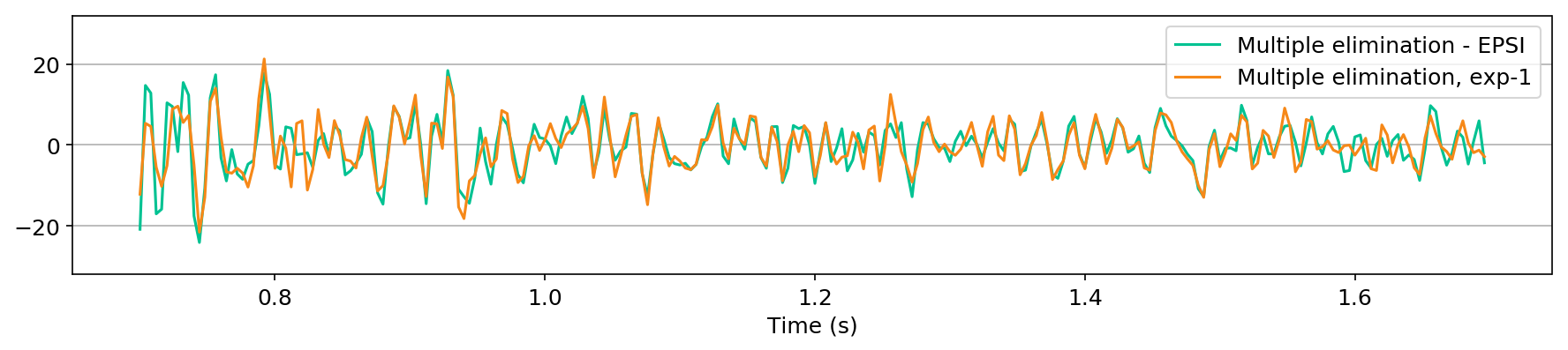
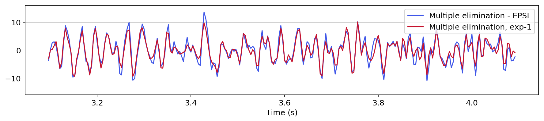
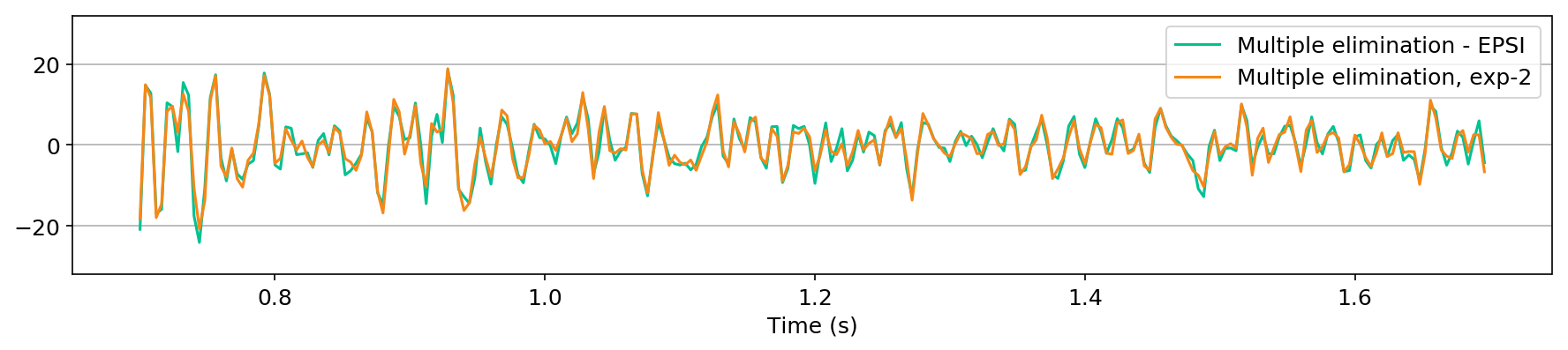
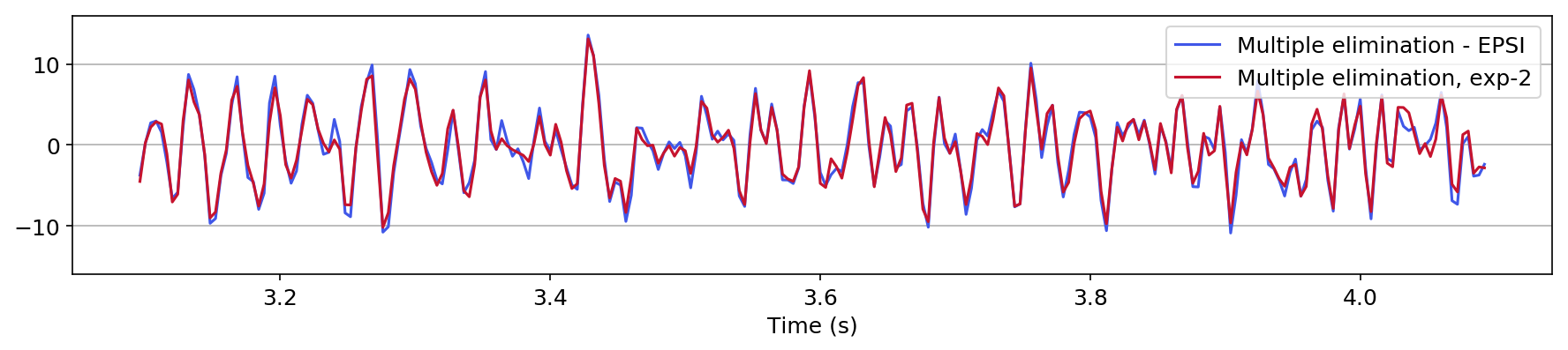
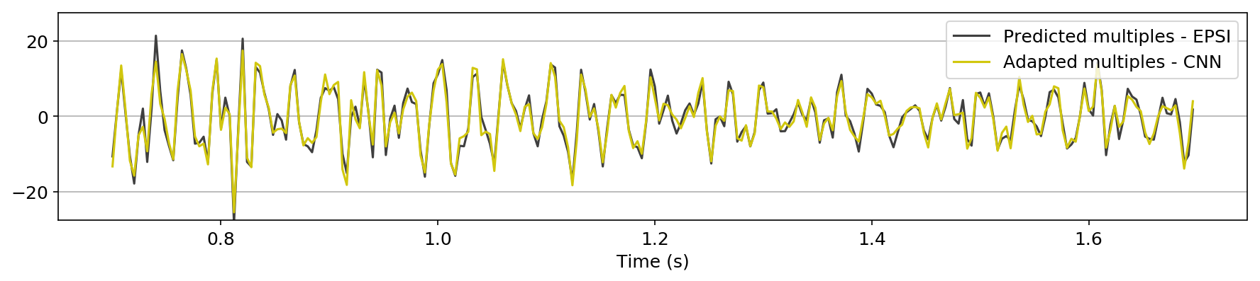
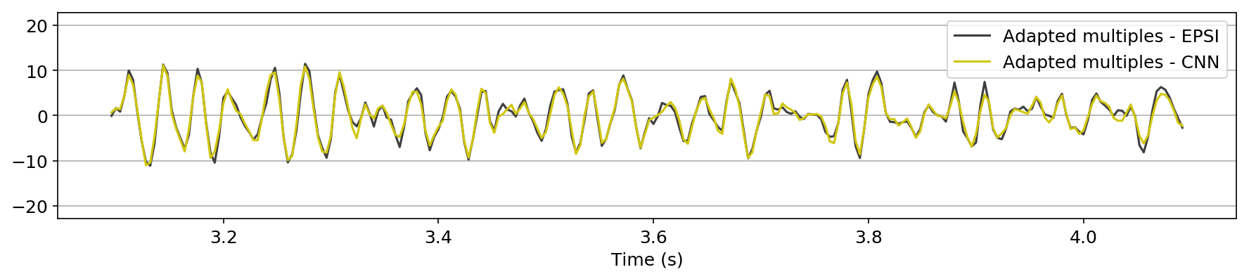
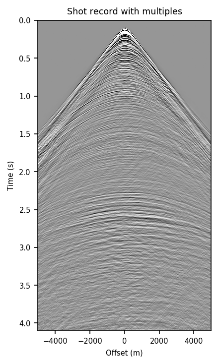
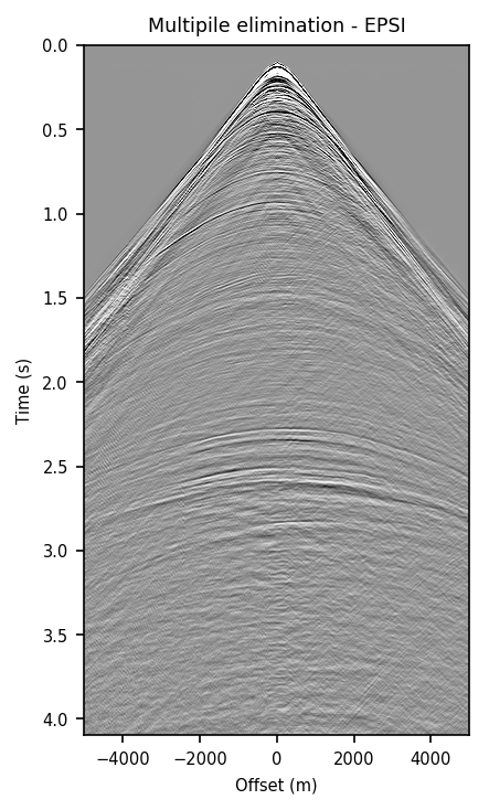
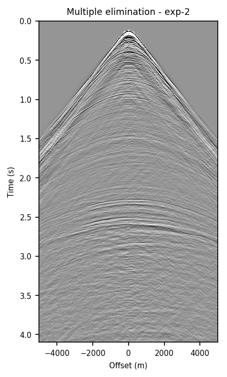
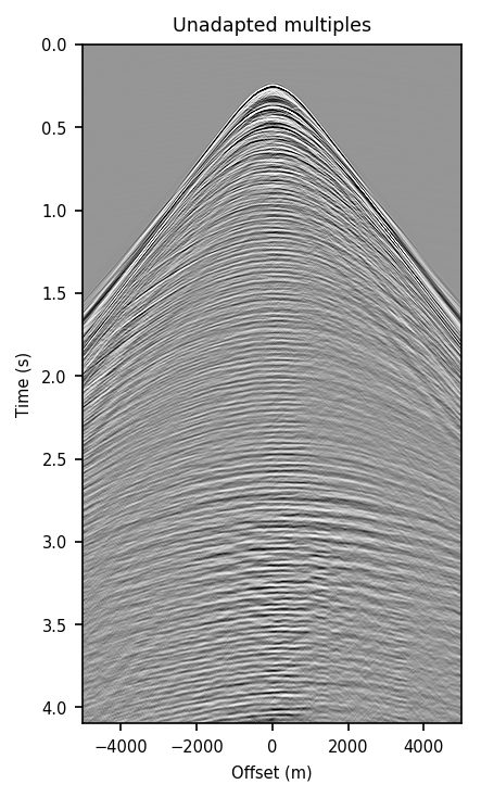
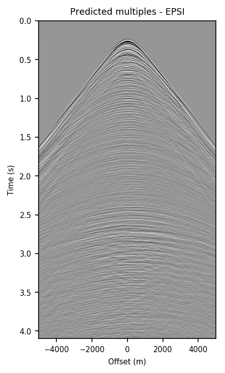
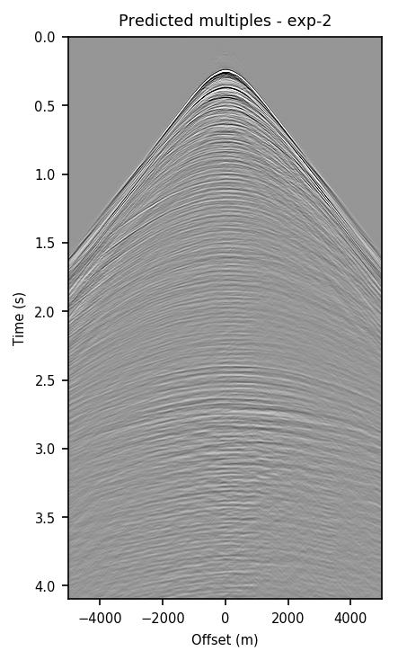
Figure 2 contains shot records and results that correspond to the zero-offset traces shown above. Figure 2a shows a shot record with surface-related multiples from Nelson data set. Figure 2b includes the same shot record but after multiple elimination via EPSI. Figures 2c and 2d depict the shot records after multiple elimination via CNNs trained according to experiments one and two. Figure 2e illustrates the predicted multiples obtained via multi-dimensional convolution of data with itself, used as an input in experiment two. Figure 2f depicts the predicted multiples via EPSI. Figure 2g contains the predicted multiples in experiment one, which is computed by subtracting the predicted primaries (Figure 2c) from the total data (Figure 2a). Finally, Figure 2h illustrates the predicted multiples via CNN trained according to experiment two.

Figure 2 demonstrates the ability of a well-trained CNN to approximate results obtained by the computationally expensive EPSI algorithm, provided suitable training data. Additionally, by comparing Figures 2c and 2g with Figures 2d and 2h, we conclude that providing the CNN with poor prediction of multiples increases the accuracy of the CNN in the second experiment. For instance, in Figure 2g, indicating predicted multiples in experiment one, we can notice leakage of first primary, errors in positioning of large offset event, and missing backscattered multiples. Note that the number of unknowns in the networks in the two experiments are slightly different because the dimensions of input/output in the second experiment is larger and consequently, it may need more training time. Although we have fixed the training time for the two experiments, results obtained via CNN in the experiment two are more accurate. The training time in both experiments is \(15.5\) hours. The average time it takes to evaluate the output of the CNN in experiment two is \(140\) ms per shot record. This corresponds to an average of \(4\) minutes per shot record to predict primaries, taking into account the time it takes to train and apply the network. The required runtime in our experiments may not be less than the time needed to apply EPSI, but it might be computationally favorable when applied in a 3D seismic survey. Also, in case there exists pairs of raw and processed (via EPSI) shot records from a proximal survey, by pre-training a neural network on the mentioned data, we can significantly reduce the time needed to fine-tune the network to the pertinent survey (Siahkoohi et al., 2019).

Discussion & conclusions

Our numerical experiments demonstrate that, given suitable training data, a well-trained neural network is capable of providing fast approximation to the action of computationally expensive Estimation of Primaries by Sparse Inversion (EPSI) algorithm, applied to field data. An important observation we made is that by providing the CNN with a relatively cheap prediction of multiples, obtained via a single step of surface-related multiple elimination method, without source-function correction, the accuracy of primariy/multiple prediction considerably increases. Although evaluating the trained convolutional neural network is extremely fast, by taking into account the training time the proposed method may only be favorable when applied in a 3D seismic survey, where EPSI will be very expensive. This method solely gives a fast and accurate approximation to EPSI, when evaluated on shot records that are drawn from the same distribution as the training data. In the next step, by exploiting transfer learning, we are looking forward to pre-training a neural network on training pairs obtained from a proximal survey and we hope to limit the number of training pairs needed from the pertinent survey for fine-tuning.

Acknowledgments

We express our appreciation to PGS for providing the Nelson field data.