Deep-learning based ocean bottom seismic wavefield recovery

Ali Siahkoohi¹, Rajiv Kumar², and Felix J. Herrmann^1
1School of Computational Science and Engineering, Georgia Institute of Technology,
²Formerly Georgia Institute of Technology; Currently DownUnder GeoSolutions, Perth, Australia

SUMMARY

Ocean bottom surveys usually suffer from having very sparse receivers. Assuming a desirable source sampling, achievable by existing methods such as (simultaneous-source) randomized marine acquisition, we propose a deep-learning based scheme to bring the receivers to the same spatial grid as sources using a convolutional neural network. By exploiting source-receiver reciprocity, we construct training pairs by artificially subsampling the fully-sampled single-receiver frequency slices using a random training mask and later, we deploy the trained neural network to fill-in the gaps in single-source frequency slices. Our experiments show that a random training mask is essential for successful wavefield recovery, even when receivers are on a periodic gird. No external training data is required and experiments on a 3D synthetic data set demonstrate that we are able to recover receivers for up to \(90\%\) missing receivers, missing either randomly or periodically, with a better recovery for random case, at low to midrange frequencies.

Introduction

Densely sampled wide-azimuth seismic data yields higher resolution images using current imaging techniques. Consequently, seismic data acquisition plays a major role in successful seismic imaging and inversion. In marine seismic surveys, data can be acquired either using a dynamic or static acquisition geometry. In dynamic geometries, sources and receivers are towed behind vessels, as opposed to static geometries, where ocean bottom nodes (OBN) or cables (OBC) are placed on the ocean bottom, and where seismic sources are towed behind one or more vessels. Compared to the other acquisition modalities, OBN geometries have several advantages. For instance, OBN geometries can cover a wider azimuth compared to dynamic geometries. Moreover, static geometry is less influenced by delays in surveying due to bad weather, physical obstacles such as exploration platforms and wells, and fluctuations in receiver depth caused by waves in the sea.

While ocean bottom seismic acquisition has many advantages, because of economic considerations, the nodes live on a very coarse grid. On the other hand, relying on existing work on randomized marine acquisition (Kumar et al., 2015; Cheng and Sacchi, 2015), we can safely assume that sources are finely sampled. Therefore, successful ocean bottom seismic acquisition relies on recovering “missing” receivers (nodes) such that the sources and receivers live on the same (spatial) grid. Recovering missing nodes is a very challenging process since the spatial sampling is large in both the inline and crossline directions. To address this problem, we present a deep-learning based methodology built on source-receiver reciprocity to recover missing receivers. This is accomplished by training a neural network to recover artificially subsampled single-receiver frequency slices, subsampled by a random subsampling mask. In other words, we rely on randomized sampling during training even if the existing receivers are sampled on a periodic grid. Although this technique is applicable to any type of receiver sampling, e.g., periodic or random, for sampling rates as low as \(10\%\), we observed better recovery when applied to randomly missing case.

Recent successes in the application of machine learning algorithms have been reported in the areas of seismic interpretation (Huang et al., 2017; Di et al., 2018; Veillard et al., 2018), seismic data processing (Siahkoohi et al., 2018b; H. Sun and Demanet, 2018; Ovcharenko et al., 2018), seismic modeling and imaging (Siahkoohi et al., 2019; Rizzuti et al., 2019; Moseley et al., 2018), and inversion (Mosser et al., 2018; Kothari et al., 2019). Several authors have addressed the seismic wavefield recovery (Siahkoohi et al., 2018a; Mandelli et al., 2018) as well. Mandelli et al. (2018) trained a neural network to jointly denoise and interpolate 2D shot records by operating on extracted patches from shot records. Siahkoohi et al. (2018a) recovered seismic wavefields by reconstructing subsampled frequency slices, by assuming that \(5\%\) of shot records are fully-sampled. We extend ideas in Siahkoohi et al. (2018a) by relaxing the assumption of having few fully-sampled shot records by exploiting reciprocity.

Our paper is organized as follows. First, we mention two organizations for monochromatic seismic data. Next, we discuss how we construct training data by using reciprocity. After a brief introduction to Generative Adversarial Networks (GANs, Goodfellow et al., 2014), we state the utilized training objective function and the Convolutional Neural Networks (CNN) architecture. Finally, we demonstrate our results on a synthetic 3D synthetic data set.

Theory

We describe how ocean bottom acquisition with fine receiver sampling can be achieved, where the receivers originally live on a coarse grid. In a typical ocean bottom acquisition geometry, sources are often subsampled mainly because of economic considerations. As mentioned earlier, we will assume sources are finely sampled on a regular periodic grid but the scheme can be applied to to geometries with irregular source sampling with simultaneous sources. Our framework operators on monochromatic frequency slices. Note that, in 3D seismic data acquisition, by working with one frequency only, we reduce the 5D seismic data (two source dimension, two receiver dimension, and one temporal dimension) into 4D. We first introduce two domains in which seismic data can be represented along the four remaining dimensions.

Matricization of monochromatic seismic data

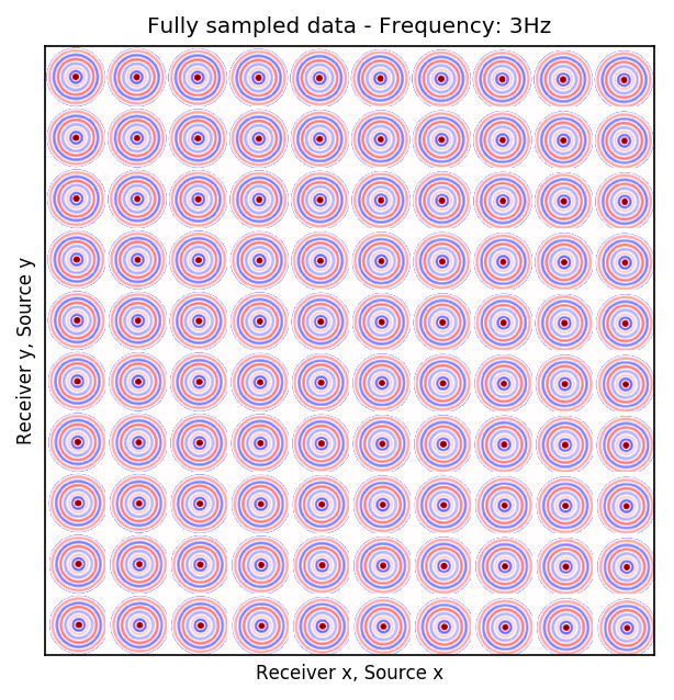
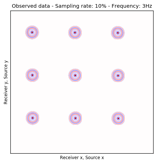
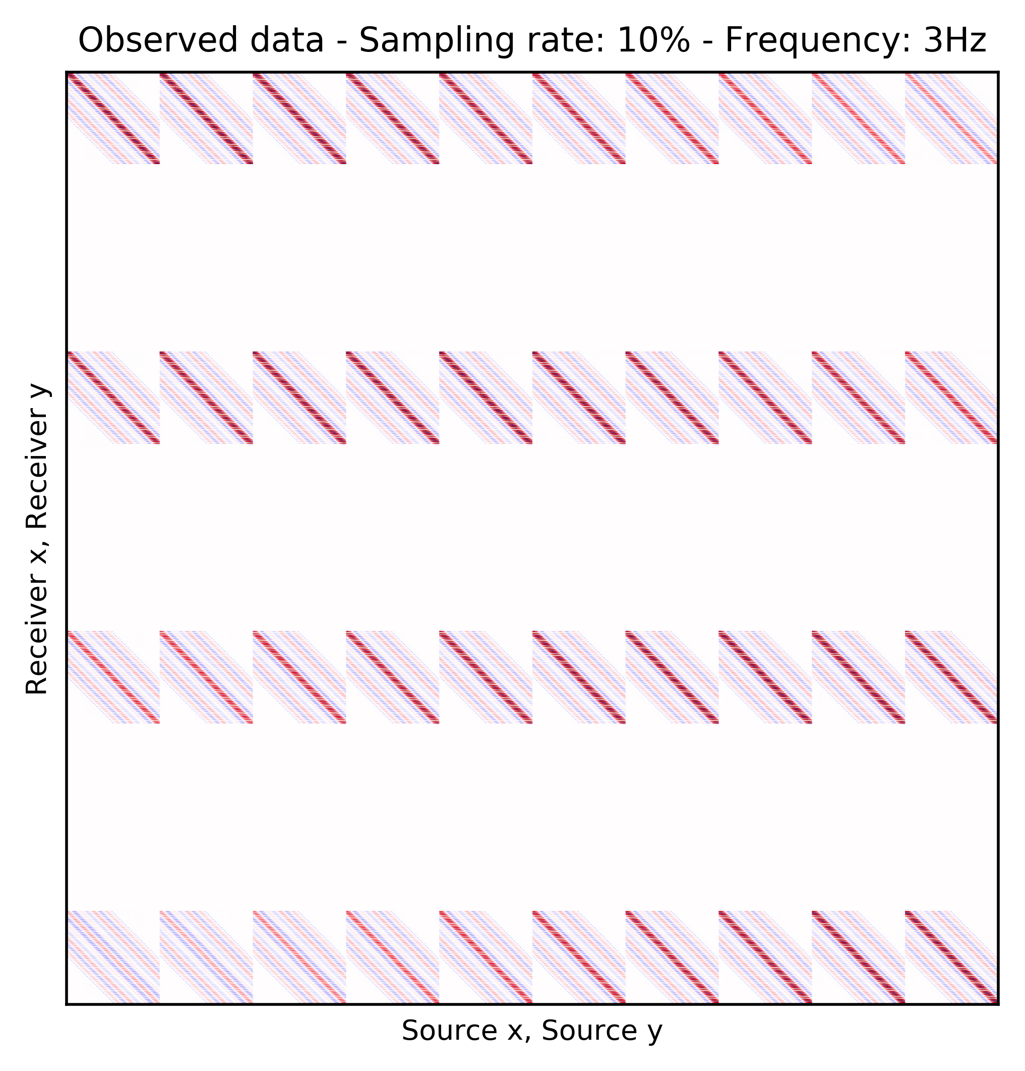
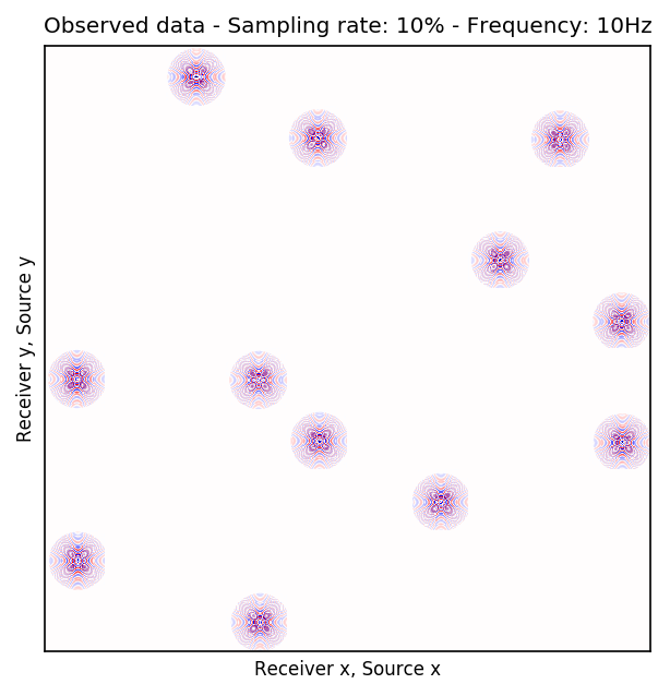
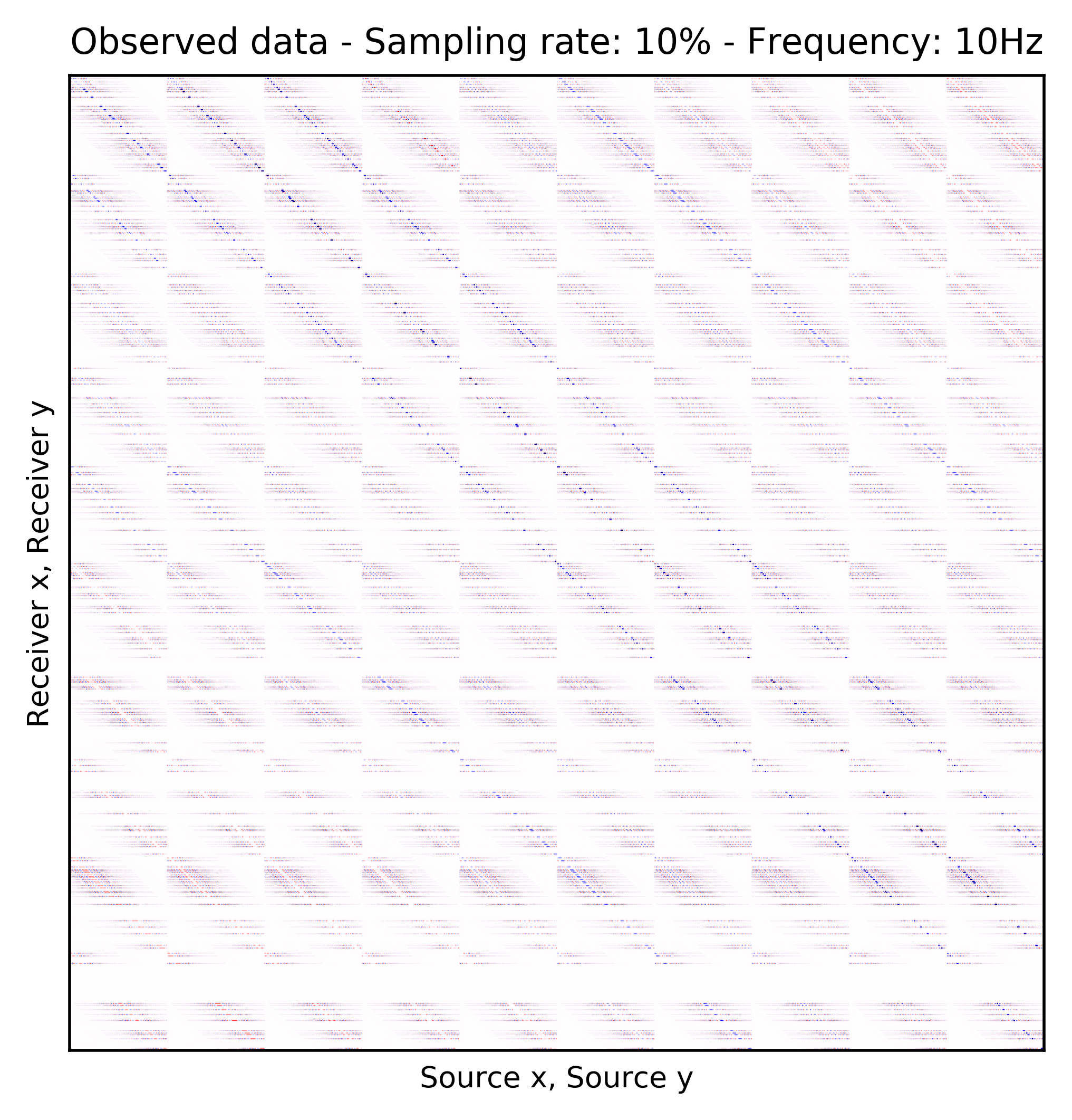
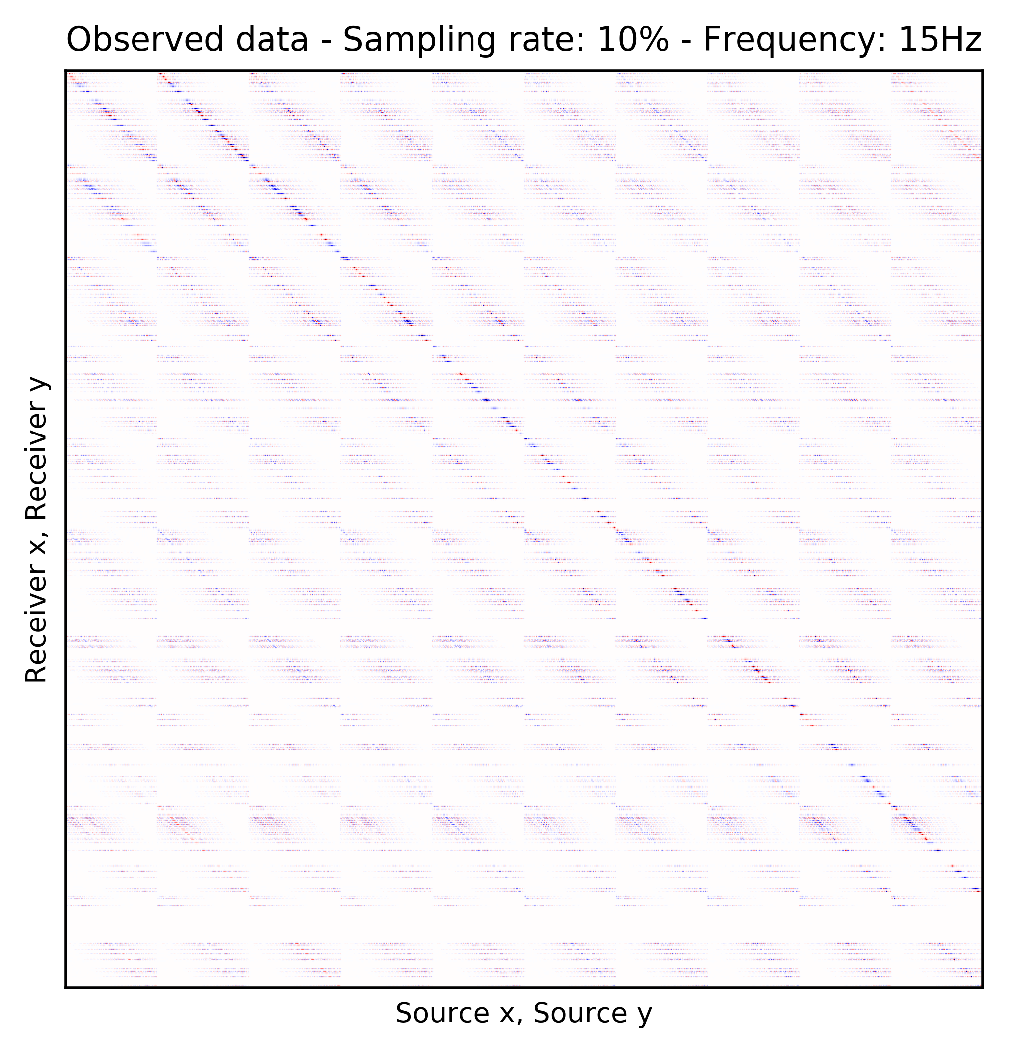
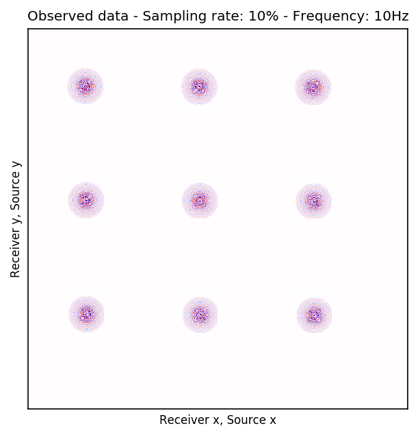
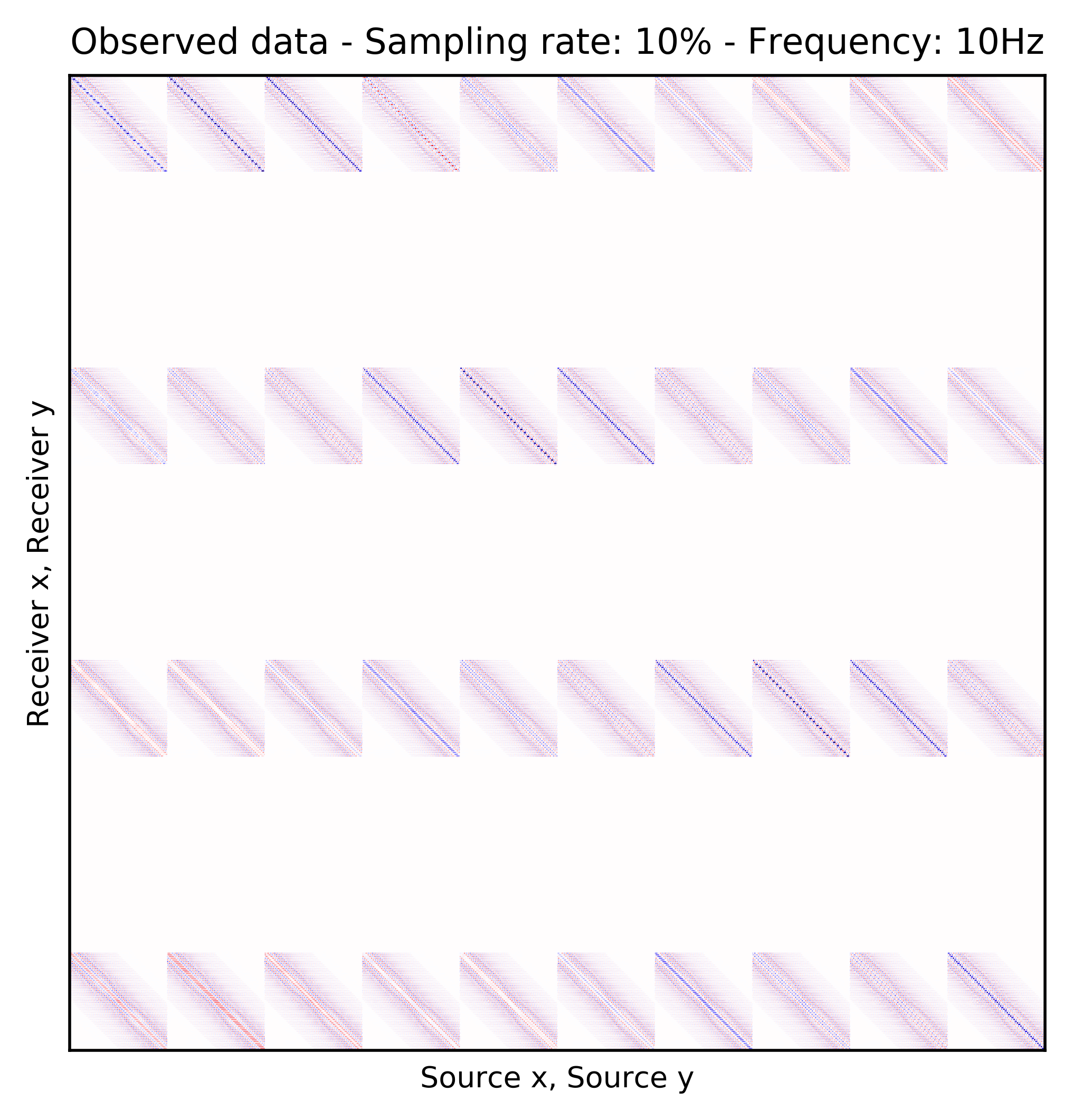
We consider single-source frequency slices as 2D complex-valued arrays of size \(N_{R_x} \times N_{R_y}\), where \(N_{R_x}\) and \(N_{R_y}\) are number of receivers in \(x\) and \(y\) coordinates, respectively. Similarly, single-receiver frequency slices are a function of two source dimensions and they can be represented as 2D complex-valued arrays of size \(N_{S_x} \times N_{S_y}\), where \(N_{S_x}\) and \(N_{S_y}\) are number of sources in \(x\) and \(y\) coordinates, respectively. There are two choices for matricization of monochromatic seismic data over the two source and receiver coordinates (Demanet, 2006; Silva and Herrmann, 2013). One matricization is obtained by putting all the vectorized single-source frequency slices in the columns of a \(N_{R_x}N_{R_y} \times N_{S_x}N_{S_y}\) array. This matricization corresponds to placing the (Rec \(x\), Rec \(y\)) dimensions in the rows and (Src \(x\), Src \(y\)) dimensions in the columns of a matrix. Evidently, the rows in this matrix correspond to vectorized single-receiver frequency slices. Another organization of seismic data in a matrix form can be obtained by placing (Rec \(y\), Src \(y\)) dimensions in the rows and (Rec \(x\), Src \(x\)) dimensions in the columns. This matrix can be considered as a matrix that includes single-receiver frequency slices as sub-matrix blocks. Suppose now that the receivers are periodically coarsely subsampled by a factor of \(10\). Figures 1a and 1b illustrate the (Rec \(y\), Src \(y\)) \(\times\) (Rec \(x\), Src \(x\)) organization of fully-sampled and subsampled monochromatic seismic data, respectively. Similarly, Figures 1c and 1d show the fully-sampled and subsampled monochromatic seismic data in (Rec \(x\), Rec \(y\)) \(\times\) (Src \(x\), Src \(y\)) organizations, respectively.

Learning to reconstruct by exploiting reciprocity

We are after bringing receivers to the same grid as sources—i.e., recovering the empty rows in Figure 1d. In order to reach this goal, we train a CNN \(\mathcal{G}_{\theta}\), parameterized by \(\theta\), consisting of all the convolutional kernels and biases. After training, the CNN takes the columns of (Rec \(x\), Rec \(y\)) \(\times\) (Src \(x\), Src \(y\)) organization—i.e., single-source frequency slices, as input and recovers the values in the gaps. Obviously, if we have such a network, we would be able to recover Figure 1c. The choice of CNN for this task is motivated by the universal approximation theorem, by Hornik et al. (1989), which states that given any continuous function defined on a compact subspace of \(\mathbb{R}^{n}\), there exists a standard feed-forward single layer neural network with enough neurons that is capable of approximating the function with arbitrary precision. Although this theorem proves the existence of such a neural network, in practice, CNNs are utilized since they are known to generalize well—i.e., maintain the quality of performance when applied to previously unseen data.

Source-receiver reciprocity holds true under certain conditions such as equal source/receiver directivity. As mentioned earlier, we want to train the CNN, \(\mathcal{G}_{\theta}\), to recover subsampled single-source frequency slices. Since receivers are severely subsampled, we do not have access to desired output for training the CNN. To address this problem, we assume source-receiver reciprocity holds—i.e., single-receiver frequency slices are reciprocal to single-source frequency slices. Therefore, to construct training pairs for the CNN, \(\mathcal{G}_{\theta}\), we artificially subsample the fully-sampled single-receiver frequency slices (non-empty rows in Figure 1d) using an arbitrary training mask. Note that we are free in choosing the training mask to subsample the fully-sampled single-receiver frequency slices. Based on our experiments, random training mask, with the same subsampling ratio as the receivers, is essential for successful wavefield recovery, even if the existing receivers are sampled on a periodic grid. Ultimately, based on source-receiver reciprocity, we hope that a well-trained CNN will perform equally well when applied to the single-source frequency slices—i.e., all columns of Figure 1d.

Generative Adversarial Networks

Let \(S_R = \left \{ \mathbf{r}_i \right \}_{i=1}^{N_R}\) be the set of fully-sampled single-receiver frequency slices, where \(N_R\) is the number of receivers actually sampled along the two receiver coordinates in the field. Denote \(S_{\hat{R}} = \left \{ \hat{\mathbf{r}}_i \right \}_{i=1}^{N_R}\) as the set of single-receiver frequency slices that are subsampled by applying a training mask to slices in \(S_R\). We use a random training mask, with the same subsampling ratio as receivers, since based on our experiments it leads to higher signal-to-noise ratio (SNR), regardless of type of receiver sampling, e.g., periodic or random. GANs introduce a framework in which the CNN, \(\mathcal{G}_{\theta}\), is coupled with an additional cnn, the discriminator, \(\mathcal{D}_{\phi}\), that learns to distinguish between fully-sampled frequency slices and the ones that have been recovered by \(\mathcal{G}_{\theta}\). Once a GAN is trained, the range of \(\mathcal{G}_{\theta}\) function will be indistinguishable from samples drawn from the probability distribution of fully-sampled frequency slices. To enforce the relationship between each specific pair of subsampled and fully-sampled frequency slices, we include an additional \(\ell_1\)-norm misfit term weighted by \(\lambda\) (Isola et al., 2017). We use the following objective function for training GANs with input-output pairs:

\[ \begin{equation} \begin{aligned} &\ \min_{\theta} \mathop{\mathbb{E}}_{\hat{\mathbf{r}}\sim p_{\hat{R}}(\hat{\mathbf{r}}),\, \mathbf{r}\sim p_R(\mathbf{r})}\left [ \left (1-\mathcal{D}_{\phi} \left (\mathcal{G}_{\theta} (\hat{\mathbf{r}}) \right) \right)^2 + \lambda \left \| \mathcal{G}_{\theta} (\hat{\mathbf{r}})-\mathbf{r} \right \|_1 \right ] ,\\ &\ \min_{\phi} \mathop{\mathbb{E}}_{\hat{\mathbf{r}}\sim p_{\hat{R}}(\hat{\mathbf{r}}),\, \mathbf{r}\sim p_R(\mathbf{r})} \left [ \left( \mathcal{D}_{\phi} \left (\mathcal{G}_{\theta}(\hat{\mathbf{r}}) \right) \right)^2 \ + \left (1-\mathcal{D}_{\phi} \left (\mathbf{r} \right) \right)^2 \right ]. \end{aligned} \label{adversarial-training} \end{equation} \]

where the expectations are approximated with the empirical mean computed with respect to pairs \((\hat{\mathbf{r}}_i,\, \mathbf{r}_i), \ i = 1,2, \ldots , N_R\) of subsampled and fully-sampled single-receiver frequency slices drawn from the probability distributions \(p_{\hat{R}} (\hat{\mathbf{r}})\) and \(p_R (\mathbf{r})\). As proposed by Johnson et al. (2016), we use a ResNet (He et al., 2016) for the generator \(\mathcal{G}_{\theta}\) and we follow Isola et al. (2017) for the discriminator \(\mathcal{D}_{\phi}\) architecture. The hyper-parameter \(\lambda\) ensures that the generator maps specific pairs \((\hat{\mathbf{r}}_i,\, \mathbf{r}_i)\) to each other (Isola et al., 2017). Solving the optimization objective \(\ref{adversarial-training}\) is typically based on Stochastic Gradient Descent (SGD) or one of its variants (Bottou et al., 2018; Goodfellow et al., 2016).

Experiments

We apply our framework to a synthetic dataset simulated on a portion of BG Compass model. The data is generated on a \(172 \times 172\) 2D periodic grid of sources and a \(172 \times 172\) 2D periodic grid of receivers, both with \(25\) m spatial sampling in both \(x\) and \(y\) directions. We will apply our algorithm to \(3\), \(5\), \(10\), and \(15\) Hz monochromatic seismic data extracted from the mentioned data set. We will evaluate the performance of the algorithm in cases where the we miss \(90\%\) of receivers, either randomly or periodic.

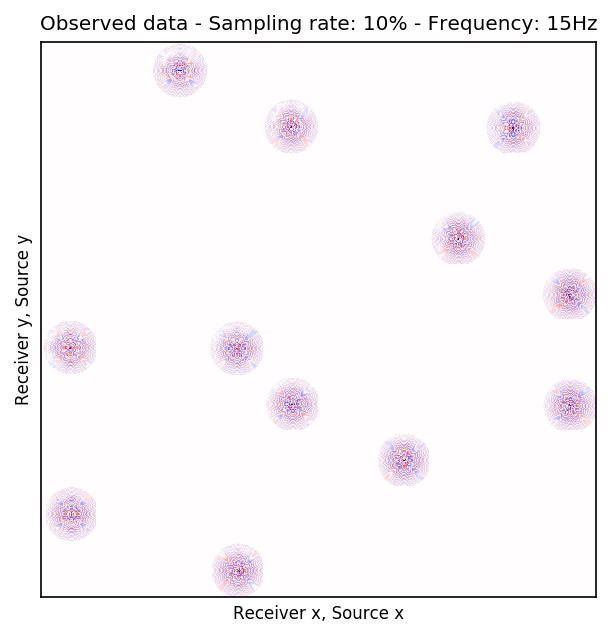
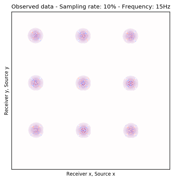
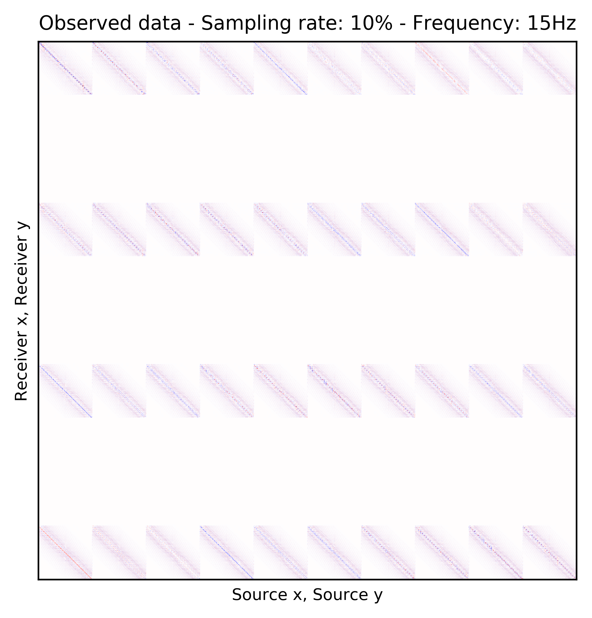
To perform our numerical experiment, we remove receivers by a factor of \(10\) for both random and periodic case. For the random case, Figures 2a and 2e in (Rec \(y\), Src \(y\)) \(\times\) (Rec \(x\), Src \(x\)) domain and Figures 2b and 2f in (Rec \(x\), Rec \(y\)) \(\times\) (Src \(x\), Src \(y\)) domain indicate the randomly picked receivers for \(10\) and \(15\) Hz, respectively. Similarly, periodically subsampled receivers for \(10\) and \(15\) Hz monochromatic seismic data in (Rec \(y\), Src \(y\)) \(\times\) (Rec \(x\), Src \(x\)) and (Rec \(x\), Rec \(y\)) \(\times\) (Src \(x\), Src \(y\)) domain can be seen in Figures 2i, 2m, 2j, and 2n. For the sake of clarity, we are only showing a small portion of the data in Figure 2 since the dimensions of the monochromatic seismic data in both matricizations is \(29584 \times 29584\). Since only \(10\%\) of the receivers are recording, we only have \(2958\) training pairs of fully-sampled and artificially subsampled single-receiver frequency slices, obtained by using a random training mask. For each frequency, we trained a CNN by minimizing Equation \(\ref{adversarial-training}\) for \(100\) passes over \(2958\) training pairs using \(\lambda = 1000\), which balances generator’s tasks for fooling the discriminator and mapping specific pairs \((\hat{\mathbf{r}}_i,\, \mathbf{r}_i)\) to each other.

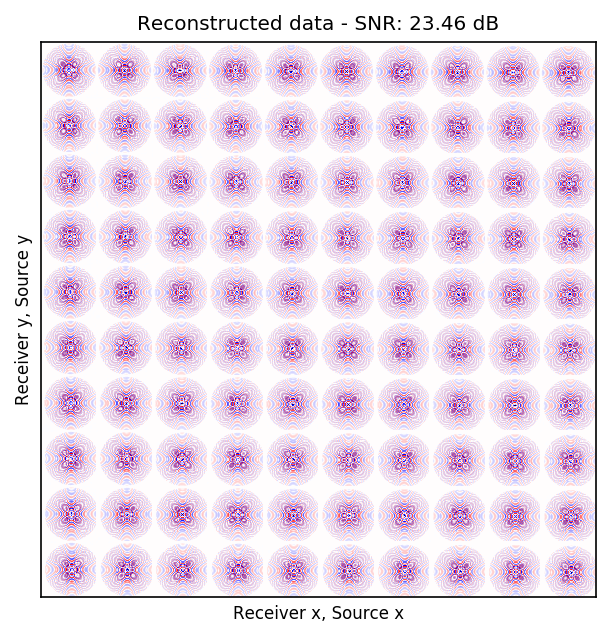
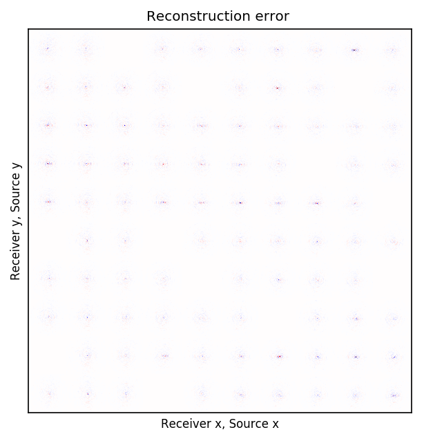
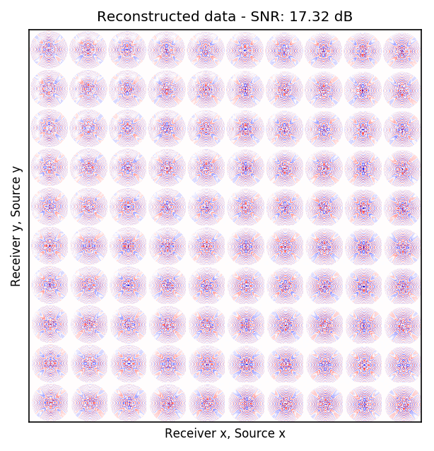
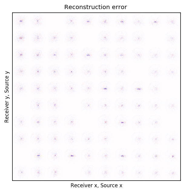
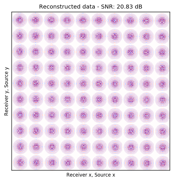
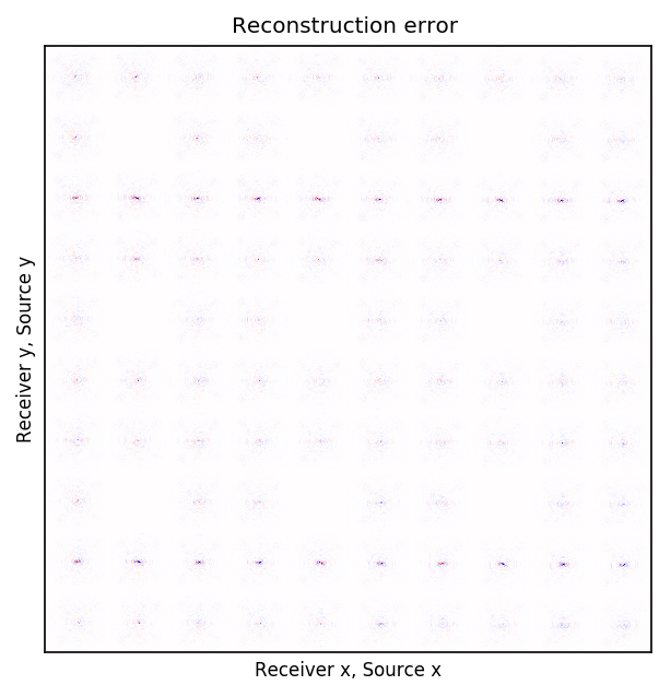
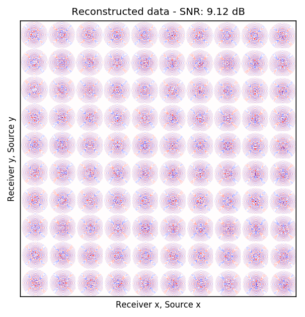
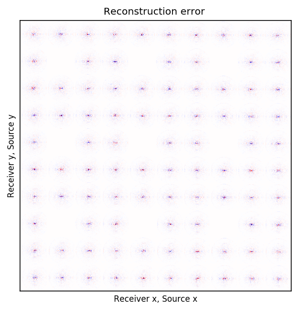
After training the CNN, for each frequency, we reconstruct the missing receivers by first, extracting single-source frequency slices from all the columns in the (Rec \(x\), Rec \(y\)) \(\times\) (Src \(x\), Src \(y\)) organization (see Figures 2b, 2f, 2j, and 2n). Next, we feed the extracted single-source frequency-slices to the trained CNN. Based on source-receiver reciprocity, we can be optimistic that the CNN will perform well when applied to the single-source frequency slices. Figures 2c, 2g, 2k, and 2o illustrate the reconstructed single-receiver frequency slices in (Rec \(y\), Src \(y\)) \(\times\) (Rec \(x\), Src \(x\)) domain for \(10\) and \(15\) Hz monochromatic seismic data, for the random and periodic case, respectively. The reconstruction error for \(10\) and \(15\) Hz are included in Figures 2d, 2h, 2l, and 2p, respectively.

The obtained results indicate that the CNN trained on pairs of fully-sampled and subsampled single-source frequency slices is able to recover the single-source frequency slices with \(90\%\) missing receivers, either missing randomly or periodically, with higher accuracy in randomly missing case. Our experiments showed that a CNN trained on training pairs obtained by subsampling the single-receiver frequency slices with a random training mask equal to the randomly missing receiver sampling mask, performs better than using a periodic training mask on both randomly and periodically missing receivers cases. While we can not fully justify this observation, but we know from Compressive Sensing that by utilizing a randomized sampling, the underlying signal can be recovered with a higher probability. We make a similar observation in our experiment, namely as the frequency increases, the performance of the method degrades faster for the periodically missing receiver case. In general, the decrease in SNR as frequency increases is understandable since in higher frequencies, the frequency slices are more intricate. Table 1 includes the average recovery SNRs for \(3\), \(5\), \(10\), and \(15\) Hz monochromatic seismic data for randomly or periodically missing receivers. Note that for the periodic case, we have used the same network as in the random case.

Sampling mask	Frequency	Average recovery SNR
random	\(3\) Hz	\(32.66\) dB
random	\(5\) Hz	\(29.07\) dB
random	\(10\) Hz	\(23.46\) dB
random	\(15\) Hz	\(17.31\) dB
periodic	\(3\) Hz	\(32.17\) dB
periodic	\(5\) Hz	\(28.32\) dB
periodic	\(10\) Hz	\(20.82\) dB
periodic	\(15\) Hz	\(9.12\) dB

Discussion & conclusions

We introduced a framework in which data recoded via an ocean bottom acquisition survey, can be mapped to a finer receiver sampling grid, regardless of type of receiver sampling, e.g., periodic or random. An important distinction of this contribution compared to similar works is that it does not need any external training data. This is accomplished by assuming that source-receiver reciprocity holds and the sources are densely sampled, which is possible using existing methods such as (simultaneous-source) randomized marine acquisition. Based on later assumption, single-receiver frequency slices, corresponding to existing receivers, are fully-sampled. We trained a CNN with training pairs consisting of the fully-sampled and artificially subsampled single-receiver frequency slices, where the subsampling is performed using a random training mask. Our numerical experiment on a 3D synthetic data set, with \(90\%\) missing receivers, missing either randomly or periodically, over low to midrange frequencies indicated that a random training mask is able to recover the wavefields with high SNR and in general, our method is more accurate when applied to randomly missing receivers case. In the future, more work is needed to improve the accuracy of the method on higher frequencies.