Deep Convolutional Neural Networks in prestack seismic—two exploratory examples

Ali Siahkoohi¹, Mathias Louboutin¹, Rajiv Kumar², and Felix J. Herrmann^1,2
1School of Computational Science and Engineering, Georgia Institute of Technology,
²School of Earth and Atmospheric Sciences, Georgia Institute of Technology

ABSTRACT

Deep convolutional neural networks are having quite an impact and have resulted in step changes in the capabilities of image and voice recognition systems and there are indications they may have a similar impact on post-stack seismic images. While these developments are certainly important, we are after all dealing with an imaging problem involving an unknown earth and not completely understood physics. When the imaging step itself is not handled properly, this may possibly offset gains offered by deep learning. Motivated by our work on deep convolutional neural networks in seismic data reconstruction, we discuss how generative networks can be employed in prestack problems ranging from the relatively mondane removal of the effects of the free surface to dealing with the complex effects of numerical dispersion in time-domain finite differences. While the results we present are preliminary, there are strong indications that generative deep convolutional neural networks can have a major impact on complex tasks in prestack seismic data processing and modeling for inversion.

Introduction

There have been lots of recent successes applying machine learning techniques to speech recognition and image classification (Krizhevsky et al., 2012; G. Hinton et al., 2012; Szegedy et al., 2015) including in seismic (Rawles and Thurber, 2015; Zhao et al., 2015; Mousavi et al., 2016; Y. Chen, 2017; Shafiq et al., 2018). While there is ample evidence that machine learning and deep convolutional neural networks (CNNs) in particular have or will very soon lead to major breakthroughs in “post-stack” seismic, the application of this exciting new technology to “prestack” seismic, whether this applies to seismic data processing or wave-equation based imaging and inversion is not clear. This paper aims to gain some insight into their potential.

While several efforts are currently underway to incorporate CNNs in imaging problems— by using them to parameterize prior probability density functions that serve as prior information on the model in inverse problems (Dokmanić et al., 2016); or by learning certain prox operators (read denoisers) in optimization (Sun et al., 2016; Fai et al., 2017; Mardani et al., 2017; Adler and Öktem, 2018) to name a few — the authors are not aware of studies that elaborate on the use of CNN’s in problems that involve complex and high-dimensional wave physics. Having said this there is a growing body of work incorporating ideas from machine learning into physical systems—e.g. there have been successes in the prediction of production curves from large production histories (X. Li et al., 2013; Aizenberg et al., 2016; Anderson et al., 2016) or in learning (nonlinear) physics from observed data (Brunton et al., 2016). But again, these examples do rely on extremely large training sets in combination with underlying manifolds that are (extremely) low dimensional.

This brings us to the topic of this contribution where we ask ourselves the question “what have CNNs to offer in seismic data processing and modeling for inversion?” To answer this question we explore the use of generative networks—i.e., networks that are not trained as a classifier but instead are capable of generating examples drawn from a probability distribution that may include a certain mapping. When properly trained, and therein lies of course the challenge, these generative networks can lead to remarkable results, see for instance recent work by Siahkoohi et al. (2018) where we recovered seismic data successfully from missing traces to a high degree of accuracy.

To further explore the potential of generative networks, we consider two different tasks for which we do have an answer namely, removal of the effects of the free surface (ghost + surface related multiples) and the removal of numerical dispersion in finite-difference modeling. Both tasks serve as proxies on how CNNs can be used to deal with inadequate physics—i.e. physical systems that for some reason are not described adequately either by not including the free surface in our formulation or by violating the stability criterion of finite differences.

As the examples demonstrate, CNNs show a remarkable ability to conduct complicated tasks even when trained on different models—i.e., a different water depth for the multiples or a different part of the velocity model for the dispersion. We feel that this opens exciting new possibilities to rethink how we formulate our problems.

We organize our work as follows. We first give a brief introduction to CNNs followed by a detailed discussion on the application of CNNs to the removal of the effects of the free surface and numerical dispersion effects in modeling.

Theory

In general, for given parameters \(\theta\), CNNs consist of several layers where within each layer the input is convolved with multiple kernels, followed by either up or down-sampling, and the elementwise application of a non-linear function (e.g. thresholding …). Let\(\ Z_0 \in \mathbb{R}^{m_0 \times n_0 \times k_0}\) be the input to the first layer. The \(i^{\text{th}}\) layer with input \(Z_{i-1}\) and output \(Z_{i}\) of a CNN consisting of \(N\) layers is given by: \[ \begin{equation} \begin{aligned} Z_{i}^{(j)} &\ = h \left ( \left( A_i^{(j)} \circ S_i \right ) \ast Z_{i-1} + B_i^{(j)} \right) \ \ \text{for} \ \ j=1, \cdots, k_{i}, \\ \ i &\ = 1, \cdots , N. \end{aligned} \label{four} \end{equation} \] where for all \(j\) in \(i^{\text{th}}\) layer, \(\ A_i^{(j)} \in \mathbb{R}^{r_i \times s_i \times k_{i-1}}\) is the\(\ j^{\text{th}}\) convolution kernel,\(\ k_{i}\) is the number of kernels and kernels only slide over the first two dimensions during convolution. \(S_i\) is an up or down-sampling operator,\(\ B_i^{(j)} \in \mathbb{R}^{m_{i} \times n_{i} }\) is\(\ j^{\text{th}}\) bias variable with same size as the result of convolution, and\(\ h\) is the elementwise non-linear function. The output of\(\ i^{\text{th}}\) layer is \(Z_{i} = [Z_{i}^{(1)}, Z_{i}^{(2)}, \cdots, Z_{i}^{(k_{i})}] \in \mathbb{R}^{m_{i} \times n_{i} \times k_{i}}\) where the size of the third dimension of the output is equal to the number of convolutional kernels used in \(i^{\text{th}}\) layer. The operator\(\ S_i,\) in case of down-sampling, performs the convolution with more than one shift in all directions. In the case of up-sampling, it periodically puts zeros between samples of\(\ Z_{i-1}\) and then performs the convolution with usual one shift. The set of parameters \(\theta\) for the described CNN consists of the convolution kernels and biases in all the layers of CNN. During training, for given input and output pairs, \(\theta\) gets optimized.

We implemented our algorithm in TensorFlow (Abadi et al., 2016) and used Devito (Lange et al., 2017; Louboutin et al., 2017) to solve the wave equation using finite difference method.

Experiments

It is obvious that there are many potential areas where CNNs could be employed in seismic data processing and modeling for inversion. As a first example to demonstrate the potential of CNNs, we select removal of the free surface effects because this problem is well understood and widely studied. Our goal here is to see whether a CNN can learn the mapping from data generated with a free surface to data without a free surface. Since the effects of the free surface only depend on the free surface itself, we expect the network to in principle generalize well—i.e., to work on data generated from a different velocity model.

As a second example, we study a possible map from numerically dispersed solutions of the wave equation to non-dispersed solutions. While a solution for this problem exists, namely modeling with sufficient numbers of gridpoints per wavelength, we are interested to see whether a trained CNN is capable to perform this far from trivial task.

Disclaimer. We are fully aware that powerful solutions exists for both tasks and it is not our claim to say we can do better or that this will ever work competitively in practice. We are merely interested in exploring potential capabilities of CNNs in prestack seismic data processing and modeling for inversion.

Example 1. Removal of the free surface

We train our CNN on shot records generated with a quasi-oracle velocity model (a training model close to the actual model) that has 25 meters difference with the oracle (= true velocity model) velocity in the water depth. In order to learn the relationship between the primaries and multiples and ghosted and deghosted data, we need to have shot records both with and without a free surface in our training dataset. Training is done over all 401 shots and we pass twenty times over the entire dataset. While we see all shots, we are training on a velocity model with a significantly different water depth.

Once the training is finished, our CNN maps a shot from the 2D dataset generated with a free surface to a shot without a free surface in about 1.8 seconds. This is very fast if we exclude the time it took to train the CNN, which is of the same order as estimation of primaries by sparse inversion.

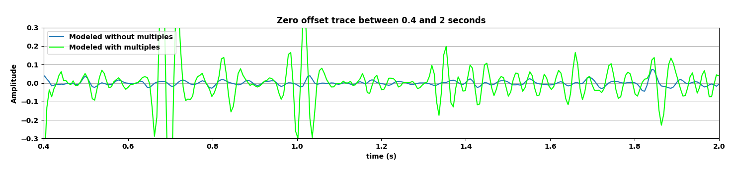
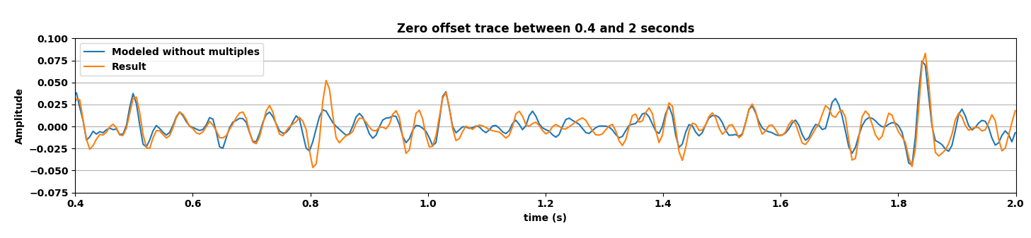
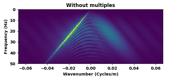
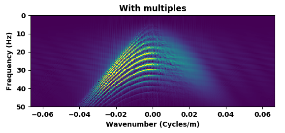
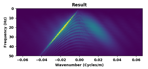
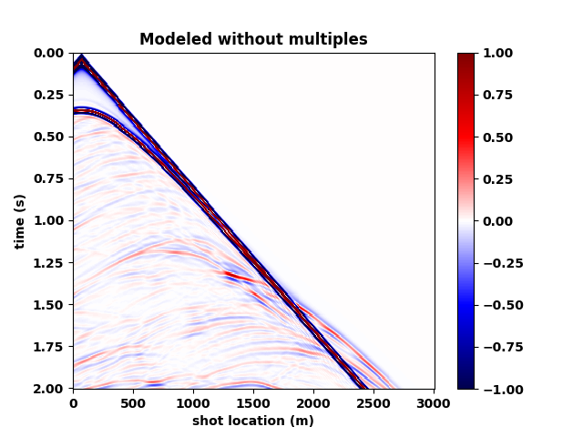
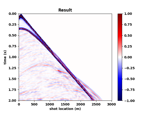
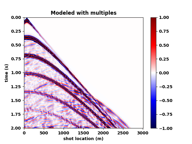
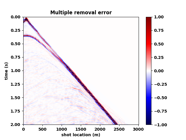
Figure 5 summarizes our results by showing the data without and with the free surface and with direct waves included. Figure 5b contains the output of the trained network mapping data generated with the free surface (Figure 5c) to data w/o a free surface (Figure 5a)—i.e., a ghost and w/o surface related multiples. Comparing the mapped data to the modeled data w/o a free surface shows that the CNN did a remarkable good job, an observation supported by the difference between the modeled and mapped data w/o a free surface (Figure 5d); the trace comparisons in Figure 1, and the f-k spectra in Figure 2. Aside from removing most of the multiple energy, the CNN also restores the low-end of the spectrum. However, the mapped result (juxtapose the two top figures of Figure 5) are certainly not perfect. We miss energy from the strong Ocean bottom reflection; from the direct wave; and from areas where there are conflicting dips (late arrival times and far offsets). Having said that these results are certainly encouraging because they were obtained more or less out of the box. We also need to remember that we are are also deghosting the data.

Example 2. Removal of numerical dispersion

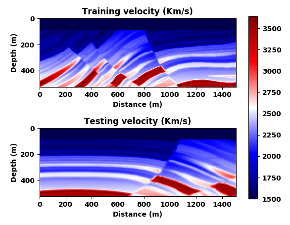
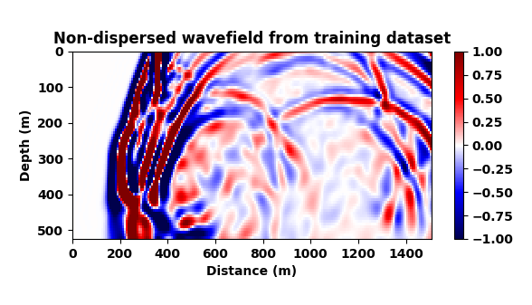
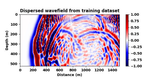
While the results of the previous example are certainly encouraging, deghosting and surface-related removal are relatively mundane operations compared to modeling for inversion that involves the solution of the wave equation. We use the term “modeling for inversion” to underline that we are often working with modeling kernels that are designed to fit observed data during an iterative inversion process. For obvious reasons, wave-equation based inversions are built on the premise that our simulations for inversion capture the physics accurately, an assumption that may not always be justified. To mimic situations where we are not capturing the right physics, we simulate waves in acoustic models (depicted in Figure 3) with only a two-point spatial finite difference stencil. By doing this, we deliberately violate the stability criterion of this numerical approximation of the wave equation. Because of this violation, we expect this low-fidelity approximation to be dispersive compared to high-fidelity simulations carried out with a 20-point stencil in the spatial directions (cf. Figures 6a and 6b).

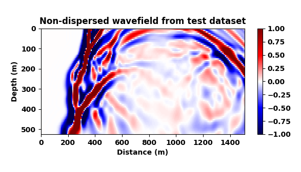
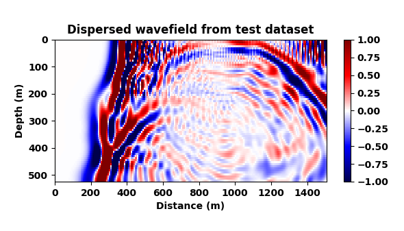
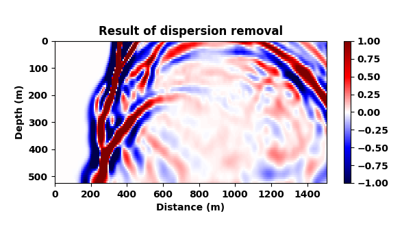
Our goal now is to train a CNN to map dispersed wavefields to non-dispersed wavelfields, a task that is not simple given the complexities of the wavefields and the non-trivial imprint of numerical dispersion. To make things more difficult and also more realistic, and to make sure the CNN is not simply memorizing what the correct non-dispersed wavefield should look like, we train the network on a different velocity model from the same geological area. To this end, we extract two slices from the 3D Marmousi model that — aside from having different water depths (this is where expect a lot of dispersion) — exhibit a completely different velocity structure albeit they were both drawn from the same geological area. We use the velocity model in Figure 3 (top) to train the CNN on pairs of wavefields (Figure 6a and 6b) and then test the trained CNN on wavefields generated from Figure 3 (bottom).

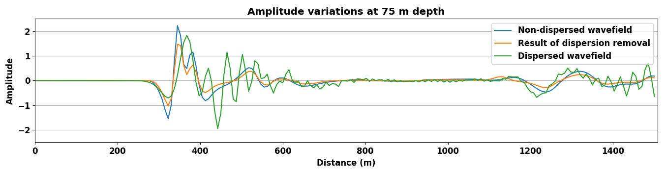
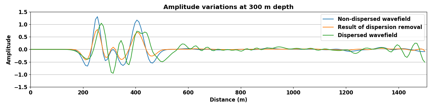
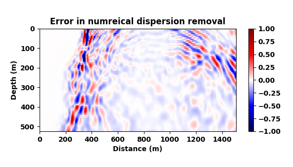
A representative time-snapshot of the non-dispersed high-fidelity test data is plotted in Figure 6c. Its low-fidelity counterpart is plotted in Figure 6d and shows, as expected, a heavy imprint of numerical dispersion. In Figure 6e, we plot the mapped result by the CNN. While certainly not perfect (see also Figure 4), the CNN demonstrates a remarkable ability to carry out this non-trivial mapping even through it was trained on a different velocity model. While there are differences in the amplitude, the phase of the different events in this complex wavefield are mostly restored and the detrimental effects of the numerical dispersion is indeed removed.

Discussion & conclusions

While it still early days on the application of deep convolutional neural networks to “pres-stack seismic”, we feel that the examples included in this work indicate that this technology has the potential to be truly transformational. Of course its eventual success will depend on our ability to train the networks; to define networks that scale to large problem sizes and that can handle noise; and above all to come up with networks that generalize to a sufficient degree. If we succeed in meeting these goals, there is no doubt in our minds that this technology will have the potential to completely revolutionize seismic data processing and inversion. Not only will we be able to remove certain unwanted components from the data (e.g. multiples + ghosts) but we will also be able to handle situations where we only have access to low-fidelity physics to carry out our inversions.

While pedagogical, the numerical dispersion example has clearly demonstrated to us that neural networks can compensate for unmodeled intricate physics. This means that as long as we are able to keep things “simple but not too simple” to quote Albert Einstein, we are in a position to make great strides forward by using networks to handle the often intractable intricacies of geophysical data while we focus on extracting valuable and interpretable information on the leading order physics. We have to say these are exciting times.

Acknowledgements

This research was carried out within Georgia Institute of Technology, School of Computational Science and Engineering.