![]()
![]()
Abstract
In this paper, we present a cost-effective low-rank factorized form of computing the full subsurface extended image volumes without explicitly calculating the receiver wavefields. The propose approach is computationally feasible, which exploits the low-rank structure of full subsurface extended image volumes organized as a matrix, thus avoiding the customary loop over sources. Using carefully selected stylized examples, we show how conventional migration images can be extracted from the low-rank factorized form. We also present a velocity continuation procedure that uses the same low-rank form and allows us to map the extended image for one velocity model to another velocity model without recomputing all the source wavefields.
Introduction
Extended image volumes contain rich sources of information, which can aside from creating images for arbitrary subsurface offset be used for the inference of rock properties, velocity analysis, and redatuming in areas of complex geology (W. W. Symes, 2008; Vasconcelos et al., 2010). Traditionally, subsurface offset or angle gathers are formed by taking multidimensional correlations of the source and receiver wavefields, as a function of all subsurface offsets (see Sava and Vasconcelos, 2011, and references therein for a recent overview). If we use a kinematically correct velocity model to form the full subsurface extended image volume, then the energy in this image volume is mainly focused at zero offset. This observation forms the basis of many migration velocity analysis schemes, where velocity model updates are calculated by minimizing an objective function that focusses the energy at zero subsurface offset (Sava and Biondi, 2004; Shen and Symes, 2008, and many others).
Unfortunately, it is computationally infeasible to compute and store extended images for all subsurface offsets and all subsurface points. For example, in 2D seismic data acquisition, the monochromatic full subsurface extended image volume is a 4-dimensional object. Moreover, in classical methods, we need to loop over all the shots to compute the source and receiver wavefields, which can easily become computationally prohibitively expensive. Therefore, the image gathers are typically only computed for a limited number of subsurface points and for a limited range of subsurface offsets, which may cause problems in complex geological areas with large geologic dips.
To overcome this computational and memory bottleneck, van Leeuwen and Herrmann (2012) proposed to probe full subsurface offset extended image volumes for information by computing the action of these image volumes on vectors that can be encoded with a certain subsurface position. By doing this, the authors avoided the expensive operation of looping over all sources by only evaluating two partial differential equations (PDEs) for each subsurface point to form a full subsurface offset image volume corresponding to that subsurface point, thus making it computationally more feasible. van Leeuwen et al. (2016) further showed the advantages of using the random Gaussian probing vectors to perform wave-equation migration velocity analyses without requiring prior information on the geologic dips.
Although probing techniques circumvent the computational bottleneck of extracting information from the full subsurface offset extended image volumes, we only have very limited access to the information from these volumes because we are restricted to the physical locations of the probing vectors. If we want to form the full subsurface extended image volumes for all the subsurface points then we have to use the classical methods to form the image volume, which can as we mention before become prohibitively expensive especially for industrial scale problems in 2D and 3D. To overcome this, we propose to exploit the low-rank structure of the monochromatic full subsurface extended image volumes organized as a matrix, where low-rank structure refers to a fast decay of the singular values. To accomplish this, we propose a randomized singular value decomposition (Halko et al., 2011) that gives us the needed low-rank factorized form of full subsurface extended image volumes. We will show that using the randomized singular value decomposition, we can form the full subsurface extended image volumes for all the subsurface offsets and all subsurface points where the cost of required PDE solves is proportional to the rank of that matrix and not the number of sources. There are indications that the rank of image volume is typically lower than the rank of the data when organized as a matrix. Apart from the computational cost, the low-rank factorization also drastically reduces the memory storage that one incurs in classical shot-profile approaches. Of course, this only holds true if the image volume can be well approximated by a low-rank factorization.
The paper is organized as follows: First, we introduce the multi-dimensional correlation-based extended imaging conditions in a two-way wave equation setting. Next, we propose the randomized singular value decomposition approach to approximate full subsurface image volumes in a computationally efficient manner. We then present a low-rank factorization based velocity continuation procedure that enables us to map the full subsurface extended image volumes from one velocity model to another velocity model at small additional cost without looping over all the sources. Finally, we demonstrate the efficacy of the proposed approach to extract various subsurface attributes (e.g. a classical RTM image). We also perform velocity continuation on Marmousi model (Brougois et al., 1990) with this approach.
Full subsurface extended image volume
We start with a brief overview of full subsurface offset extended image volumes for all subsurface points. Let \(\mathbf{U}\) and \(\mathbf{V}\) represent the monochromatic forward and adjoint wavefields, which are obtained by solving \[ \begin{gather} \label{forward} \mathbf{H}(\mathbf{m})\mathbf{U} = \mathbf{P}_s^\top \mathbf{Q},\\ \label{adjoint} \mathbf{H}^*(\mathbf{m})\mathbf{V} = \mathbf{P}_r^\top \mathbf{D}. \end{gather} \] Here \(\mathbf{H}(\mathbf{m})\) is a discretization of the Helmholtz operator with absorbing boundary conditions, \(\mathbf{m}\) is the gridded squared slowness; the matrices \(\mathbf{P}_s, \mathbf{P}_r\) restrict the full subsurface wavefields at the source and receiver locations. Finally, the symbols \(^\top\) and \(^*\) denote matrix transpose and conjugate-transpose, receptively. The \(N_s \times N_s\) matrix \(\mathbf{Q}\) contains the source weights, where \(N_s\) is the number of sources. Similarly, the \(N_r \times N_s\) matrix \(\mathbf{D}\) represents monochromatic frequency slice, where each column is a single source experiment, and \(N_r\) denotes the number of receivers.
Following van Leeuwen and Herrmann (2012), we denote the full subsurface monochromatic extended image volume as \[ \begin{equation} \mathbf{E} = \mathbf{V}\mathbf{U}^*. \label{EIV} \end{equation} \] By substituting equations \(\ref{forward}\) and \(\ref{adjoint}\) into equation \(\ref{EIV}\), we can rewrite \(\mathbf{E}\) as a function of \(\mathbf{Q}\) and \(\mathbf{D}\) as follows: \[ \begin{equation} \mathbf{E} = \mathbf{H}^{-*}\mathbf{P}_r^\top \mathbf{D}(\mathbf{H}^{-1}\mathbf{P}_s^\top \mathbf{Q})^{*}. \label{EIVT} \end{equation} \] Practically, we can never hope to evaluate equation \(\ref{EIVT}\) to form matrix \(\mathbf{E}\) since it requires \(2N_s\) wave-equation solves. Moreover, we need to store a dense \(N_x \times N_x\) matrix, where \(N_x\) represents the total number of grid points. Clearly, this is a very large object especially in 3D suggesting a need to exploit possible redundancies living in these volumes.
Our aim now is to build the accurate representation of the extended image volumes for the reasonable cost in memory storage and computational time. To achieve this, we analyze the decay of the singular values of the full subsurface extended image volumes. We are particularly interested to see whether these singular decay fast so that these volumes can be approximated accurately by a rank \(r\) matrix. Note that the rank of \(\mathbf{E}\) is at most \(N_s\) (due to equation \(\ref{EIV}\)) so we are looking for approximation with \(r\ll N_s\) singular vectors.
Low-rank factorization of image volumes
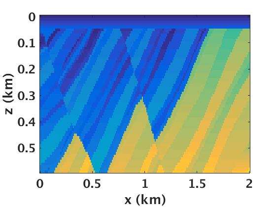
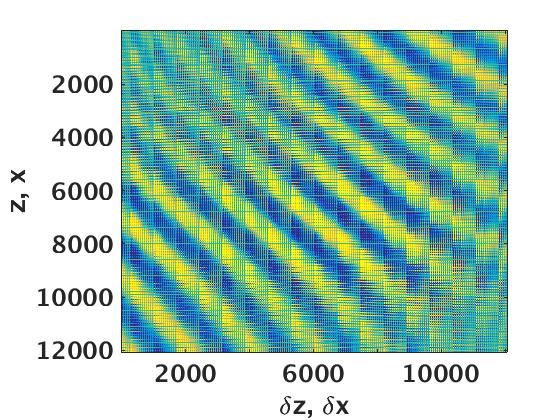
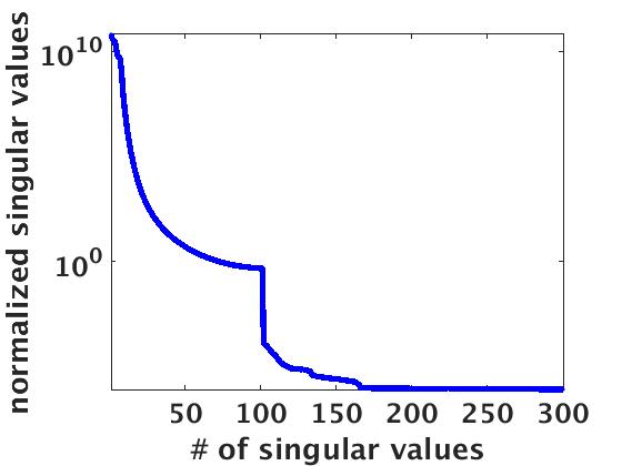
To illustrate that image volumes indeed permit low-rank factorizations at low to mid range frequencies, we analyze \(\mathbf{E}\) on a small but geologically complex subset of the Marmousi model, which consists of strongly dipping reflectors and strong lateral variations (Figure 1a). The velocity model is \(0.6\,\mathrm{km}\) deep and \(2\,\mathrm{km}\) wide, sampled at \(5\,\mathrm{m}\). The synthetic data consists of \(100\) sources and receivers sampled at \(10\,\mathrm{m}\), respectively. Figure 1b shows the full subsurface image volume matrix at \(5\,\mathrm{Hz}\) and Figure 1c displays its associated singular values decay. We can clearly see the fast decay of the singular values, which suggest that the underlying matrix of interest can well be approximated by a low-rank factorization. For instance, If we approximate the matrix \(\mathbf{E}\) with its top \(10\) singular vectors we find a signal-to-noise (SNR) ratio of about \(50\,\mathrm{dB}\). This implies that we capture most of the coherent energy with a low-rank approximation. This observation is crucial for our approach because it demonstrates that even for complex velocity models full subsurface extended image volumes exhibit a low-rank structure.
In the above example, we approximate the extended image volume \(\mathbf{E}\) by computing its top \(10\) singular vectors using the singular value decomposition (SVD). Although a naive SVD approach can compress \(\mathbf{E}\), some important limitations remain—i.e., (i) we need to solve \(2N_s\) PDEs, which are computationally prohibitively expensive for large-scale 2D and 3D, and (ii) the cost of naive singular value decomposition (SVD) of the full subsurface image volume is of the order of \(\mathcal{O}(N_x^3)\) using LAPACK based SVD algorithms (Holmes et al. (2007)).
To circumvent the computational cost of SVD, we propose to use the randomized SVD based approach (Halko et al., 2011) to compute the low-rank approximation of full subsurface extended image volumes. We emphasize that this algorithm, recalled as Algorithm 1, is significantly cheaper than computing an SVD of the full matrix. The computational cost of the proposed framework is \(4r\) PDEs, instead of \(2N_s\) PDEs, apart from computing the SVD at line 4, and a QR decomposition in line 2. Since the matrices \(\mathbf{Y} \in \mathbb{C}^{N_x \times r}\) and \(\mathbf{Z} \in \mathbb{C}^{r \times N_x}\) are tall and thin matrices, hence, computing the SVD and QR decomposition is computationally feasible and cheaper than solving the extra \((2N_s-4r)\) PDEs. As long as \(4r\ll 2N_s\), we gain orders of magnitude while computing the low-rank approximation of image volumes using the randomized SVD. Given the randomized SVD framework, we can now represent the full subsurface extended image volumes in terms of two low-rank factors, i.e. \(\mathbf{E} \approx \widetilde{\mathbf{E}} = \mathbf{L}\mathbf{R}^{*}\), where \({\mathbf{L}} = {\mathbf{T}} \sqrt{\mathbf{X}}\) and \({\mathbf{R}} = {\mathbf{F}} \sqrt{\mathbf{X}}\). This matrix factorization is much smaller than the full extended image volume, but still contains most of the energy of \(\mathbf{E}\). Hence, the randomized SVD framework is computationally feasible for large-scale 2D and 3D seismic problems.
1. \(\mathbf{Y} = \mathbf{E} \mathbf{W}\), here, \(\mathbf{W}\) is \((N_x \times r)\) Gaussian random matrix
2. \([\mathbf{N},{\mathbf{R}}] = \text{qr}(\mathbf{Y})\)
3. \(\mathbf{Z} = \mathbf{N}^* \mathbf{E}\)
4. \([{\mathbf{T}},\mathbf{X},{\mathbf{F}}] = \text{svd}(\mathbf{Z})\) (\(\mathbf{Z} \in \mathbb{C}^{r \times N_x}\) is a small matrix), where \(\text{svd}\) computes the top \(r\) singular vectors of \(\mathbf{Z}\)
5. \({\mathbf{T}} \gets \mathbf{N}{\mathbf{T}}\)
6. \({\mathbf{L}} = {\mathbf{T}} \sqrt{\mathbf{X}}\) and \({\mathbf{R}} = {\mathbf{F}} \sqrt{\mathbf{X}}\)
7. \(\mathbf{E} \approx \widetilde{\mathbf{E}} = \mathbf{L}\mathbf{R}^{*}\), here \(\mathbf{L}\) and \(\mathbf{R} \) are \((N_x \times r)\) matrices
Once we estimate the low-rank factorized form of the extended image volumes, we can extract any subsurface image attributes out of it. For example, the diagonal of the monochromatic full subsurface extended image volume corresponds to the monochromatic reverse-time migration image (RTM). To compute the conventional migration images, we can apply the zero-time/offset imaging condition as follows: \[ \begin{equation} \text{RTM} = \sum_{j=1}^{N_f} -\omega_j^2 \text{diag}(\widetilde{\mathbf{E}}_{\omega_j}) = \sum_{j=1}^{N_f}\sum_{i=1}^r -\omega_j^2 (\mathbf{L}_{\omega_j}(:,i) \odot \mathbf{R}_{\omega_j}(:,i)), \label{Diag} \end{equation} \] where \(\odot\) is the Hadamard product or the entrywise product (Davis (1962)), \(N_f\) represents the number of frequencies, and \(\omega\) is the temporal frequency . Similarly, we can extract in a computationally efficient manner common-image point gathers (CIPs) and common-image gathers (CIGs) from the factors \(\mathbf{L}\) and \(\mathbf{R}\).
Invariance formulation of image volume
Apart from extracting various subsurface image attributes from full subsurface extended image volumes, the linear algebraic structure of the extended image volumes (equation \(\ref{EIVT}\)) provide an invariance relationship with respect to the underlying velocity model. This invariance relation (van Leeuwen and Herrmann, 2012) can be used to map the extended image for one velocity model to another velocity model. To understand this, we rewrite equation \(\ref{EIVT}\) as a function of \(\mathbf{Q}\) and \(\mathbf{D}\) as follows: \[ \begin{equation} \mathbf{H}(\mathbf{m})^{*}\mathbf{E} \mathbf{H}(\mathbf{m})^{*} = \mathbf{P}_r^\top \mathbf{D} \mathbf{Q}^* \mathbf{P}_s. \label{fullEIV} \end{equation} \] Equation \(\ref{fullEIV}\) represents a generalization of the double square-root (DSR) equation, which uses a one-way approximation. We can indeed observe that, for a seismic data acquisition, the kernel on right hand side \(\mathbf{P}_r^\top \mathbf{D} \mathbf{Q}^* \mathbf{P}_s\) of equation \(\ref{fullEIV}\) remains invariant under changes of the velocity model. Thus, we can map the full subsurface extended image volume from velocity model \(\mathbf{m}_1\) to model \(\mathbf{m}_2\), which we can express as \[ \begin{equation} \mathbf{H}(\mathbf{m}_2)^{*}\mathbf{E}(\mathbf{m}_2) \mathbf{H}(\mathbf{m}_2)^{*} = \mathbf{H}(\mathbf{m}_1)^{*}\mathbf{E}(\mathbf{m}_1) \mathbf{H}(\mathbf{m}_1)^{*}. \label{IV} \end{equation} \] Although, we can map from one velocity to another, we need to solve \(2N_s\) PDEs, which is computationally expensive. To overcome these computational cost, we propose to use the low-rank factorization of the extended image volumes (Algorithm 1), and replace \(\mathbf{E}\) with \(\widetilde{\mathbf{E}}\) in equation \(\ref{IV}\) to evaluate the invariance relationship. Given the low-rank approximation of full subsurface extended image volume, i.e., \(\mathbf{L}\) and \(\mathbf{R}\), we can rewrite equation \(\ref{IV}\) as \[ \begin{equation} \mathbf{H}(\mathbf{m}_2)^{*}\mathbf{L}(\mathbf{m}_2)\mathbf{R}(\mathbf{m}_2)^{*} \mathbf{H}(\mathbf{m}_2)^{*} = \mathbf{H}(\mathbf{m}_1)^{*}\mathbf{L}(\mathbf{m}_1)\mathbf{R}(\mathbf{m}_1)^{*} \mathbf{H}(\mathbf{m}_1)^{*}. \label{IV1} \end{equation} \] Once we compute the low-rank factors of full subsurface extended image volume for any initial velocity model, we can then compute the subsequent low-rank factors for another velocity model as we describe below \[ \begin{equation} \begin{split} \mathbf{L}(\mathbf{m}_2) = \mathbf{H}(\mathbf{m}_2)^{-*}\mathbf{H}(\mathbf{m}_1)^{*} \mathbf{L}(\mathbf{m}_1), \\ \mathbf{R}(\mathbf{m}_2) = \mathbf{H}(\mathbf{m}_2)^{-*}\mathbf{H}(\mathbf{m}_1)^{*} \mathbf{R}(\mathbf{m}_1). \end{split} \label{eq-InvForm2} \end{equation} \] It is evident from equation \(\ref{eq-InvForm2}\) that we only need to solve \(2r\) PDEs to map one full subsurface extended image volume to another image volume pertaining to a different velocity model. So in effect, our low-rank factors allow us to replace the costumery loop over \(2N_s\) PDEs by a loop over \(2r\). As a result, we can use equation \(\ref{eq-InvForm2}\) to quickly scan over different velocity models without recomputing the source and receiver wavefields and the full subsurface extended image volumes.
Numerical Results
To illustrate the efficacy of the low-rank factorization of the full subsurface extended image volumes, we use a small but complex section of the Marmousi model, sampled at \(5\,\mathrm{m}\). We use a Ricker wavelet with a central frequency of \(20\,\mathrm{Hz}\), and simulate a dataset with \(301\) co-incident sources and receivers sampled at \(20\,\mathrm{m}\). We show three different examples here. The purpose of these examples is twofold: (i) demonstrate the computational and memory advantages of forming the full subsurface extended image volumes (EIV) using the proposed approach, and (ii) compare the quality of subsurface attributes, such as reverse-time migration images (RTM), as if computed using the traditional techniques.
Computational Aspects
In the first example, we report the computational time and memory usage of forming full subsurface image volumes using the classical approach and our randomized SVD (Algorithm 1). To show the benefits over the full bandwidth of the underlying signal, we extract four frequency slices from the data ranging from \(5\) to \(50\,\mathrm{Hz}\). As summarized in Table 1, the savings in computational time and memory are highly significant. For this example, we find a factor of more than 400 in time and more than 1500 in memory storage.
| frequency (\(\mathrm{Hz}\)) | real rank | full time (\(\mathrm{s}\)) | estimated rank | reduced time (\(\mathrm{s}\)) | SNR (\(\mathrm{dB}\)) | memory ratio |
|---|---|---|---|---|---|---|
| 5 | 301 | 4832 | 7 | 11 | 29 | 2100 |
| 20 | 301 | 4864 | 11 | 12 | 20 | 1380 |
| 30 | 301 | 5335 | 16 | 15 | 22 | 950 |
| 50 | 301 | 4825 | 25 | 21 | 20 | 608 |
Reverse-time migration
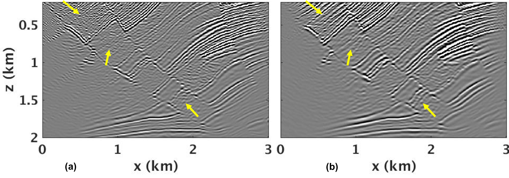
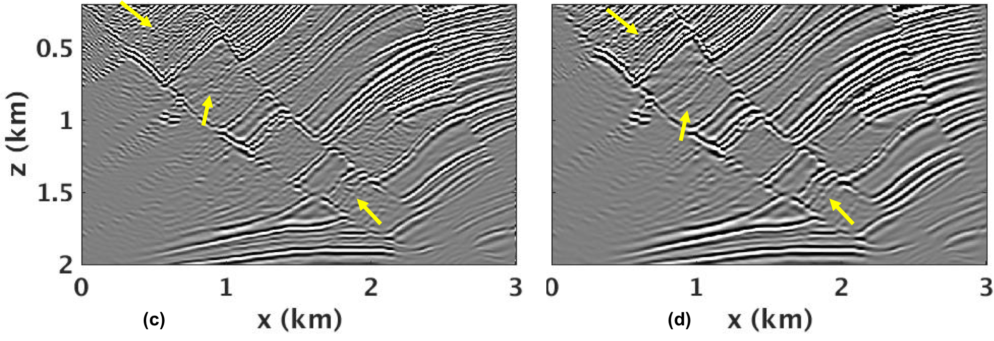
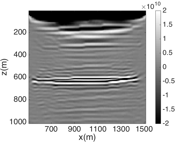
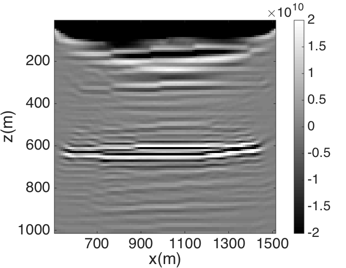
With the second example, we aim to demonstrate the benefits of performing reverse time migration with full subsurface extended image volumes, and compare these results with conventional shot-profile reverse-time migration. We again work on a subset of Marmousi model. In both cases we are interested in reducing the costs of reverse-time migration (RTM) by either working with simultaneous shots or with extended image volumes obtained by probing. For conventional RTM this corresponds to working with \(r\ll N_s\) simultaneous shots in the data space (Herrmann and Li, 2012). For the randomized SVD approach, we probe with model space simultaneous shots instead. We keep the number of PDE solves for both approaches the same, which means that the number of probing vectors for randomized SVD is half that of the simultaneous shots for conventional RTM. Figures 2(a,c) show the conventional RTM image for \(r=10\) and \(100\), respectively, whereas, Figures 2(b,d) show the diagonal of the approximated full subsurface extended image volumes for \(r=5\) and \(50\) using the randomized SVD. We can clearly see that the simultaneous sources in the classical approach create more artifacts as highlighted with yellow markers, whereas, we preserve continuity using the proposed framework. We believe that this empirical observation may have important consequences on how to solve this imaging problem. At this point we have two possible explanations for this phenomena. First, there are indications that the singular values of image volumes decay faster than the observed data organized as a matrix in the canonical organization. Second, and this is deeper argument, one can argue that the extended Born scattering operators, linking our extended image volumes to the data, are near isometries (W. W. Symes, 2008; Hou and Symes, 2016; Kroode, 2012), so migration acts more as an inverse. In either case, these results are very encouraging.
Velocity continuation
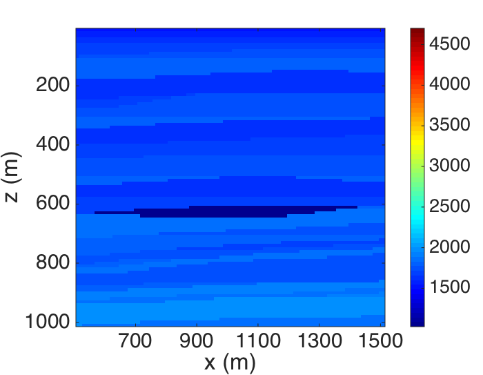
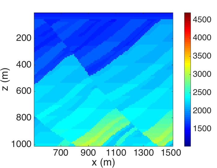
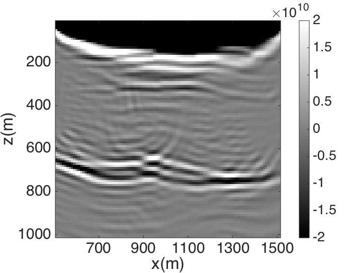
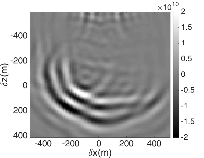
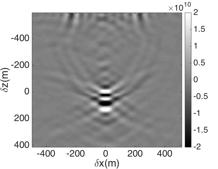
The final example illustrates advantages of the afore mentioned invariance formulation. To do so, we extract two different subsections from the Marmousi model and represent them as \(\mathbf{m}_1\) and \(\mathbf{m}_2\), where \(\mathbf{m}_1\) is the wrong initial background velocity model, and \(\mathbf{m}_2\) is the true velocity model (Figure 3). We perform the following steps to carry out velocity continuation: (i) for a fixed rank \(r\), we compute the EIV for \(\mathbf{m}_1\) and store the associated \(\mathbf{L}(\mathbf{m}_1)\) and \(\mathbf{R}(\mathbf{m}_1)\) factors, which will cost \(4r\) PDEs solves; (ii) we apply equation \(\ref{eq-InvForm2}\) to compute \(\mathbf{L}(\mathbf{m}_2)\) and \(\mathbf{R}(\mathbf{m}_2)\), which will cost \(2r\) additional PDEs, (iii) we use equation \(\ref{Diag}\) to extract the zero-offset image and compare it with the diagonal of the image volume computed directly from \(\mathbf{m}_2\) using Algorithm 1. We display the resulting RTM images in Figures 4(a,b,c) and CIP gathers in Figures 4(d,e,f). We see clearly that the initial RTM image 4(a) is far from the correct RTM image 4(c) for the true model. However, with the proposed invariance relationship, we can recover the correct image in Figure 4(b). The same observation can be made for the CIP gathers. Thus, with the extra cost of \(2r\) PDEs, instead of \(2N_s\) PDEs, we extract full subsurface image volume for any velocity model, and replace the expensive customary loops over sources in classical methods by probing with low-rank factors \(\mathbf{L}\) and \(\mathbf{R}\).

Conclusions
We presented a randomized singular value decomposition framework to get a low-rank factorized form of full subsurface extended image volumes. The proposed factorization approach exploits the linear algebraic structure of the extended image volumes, thus making it computationally feasible to form extended images for all subsurface offsets and for all subsurface points. Using the randomized singular value decomposition, we showed that the cost of required number of PDE solves is proportional to the rank of the underlying full subsurface image volumes and not the number of sources. By means of concrete examples, we demonstrated how we can extract the conventional migration images from the low-rank factorized form of the image volumes. We also proposed a cost-effective formulation to perform velocity continuation, which can be used to map the extended image for one velocity model to another velocity model.
Acknowledgements
This research was carried out as part of the SINBAD II project with the support of the member organizations of the SINBAD Consortium. M.G. would like to thank the Swiss NSF (grant P300P2-167681) for its financial support while working at SLIM, UBC.
Brougois, A., Bourget, M., Lailly, P., Poulet, M., Ricarte, P., and Versteeg, R., 1990, Marmousi, model and data: In EAEG workshop-practical aspects of seismic data inversion.
Davis, C., 1962, The norm of the schur product operation: Numerische Mathematik, 4, 343–344.
Halko, N., Martinsson, P.-G., and Tropp, J. A., 2011, Finding structure with randomness: Probabilistic algorithms for constructing approximate matrix decompositions: SIAM Review, 53, 217–288.
Herrmann, F. J., and Li, X., 2012, Efficient least-squares imaging with sparsity promotion and compressive sensing: Geophysical Prospecting, 60, 696–712. doi:10.1111/j.1365-2478.2011.01041.x
Holmes, M., Gray, A., and Isbell, C., 2007, Fast sVD for large-scale matrices: In Workshop on efficient machine learning at nIPS (Vol. 58, pp. 249–252).
Hou, J., and Symes, W. W., 2016, An alternative formula for approximate extended born inversion: Geophysics, 82, S1–S8.
Kroode, F. ten, 2012, A wave-equation-based kirchhoff operator: Inverse Problems, 28, 115013.
Sava, P., and Biondi, B., 2004, Wave-equation migration velocity analysis. I. Theory: Geophysical Prospecting, 52, 593–606. Retrieved from http://dx.doi.org/10.1111/j.1365-2478.2004.00447.x
Sava, P., and Vasconcelos, I., 2011, Extended imaging conditions for wave-equation migration: Geophysical Prospecting, 59, 35–55. doi:10.1111/j.1365-2478.2010.00888.x
Shen, P., and Symes, W. W., 2008, Automatic velocity analysis via shot profile migration: Geophysics, 73, VE49–VE59. Retrieved from http://dx.doi.org/10.1190/1.2972021
Symes, W. W., 2008, Migration velocity analysis and waveform inversion: Geophysical Prospecting, 56, 765–790.
van Leeuwen, T., and Herrmann, F. J., 2012, Wave-equation extended images: Computation and velocity continuation: EAGE technical program. EAGE; EAGE. Retrieved from https://www.slim.eos.ubc.ca/Publications/Public/Conferences/EAGE/2012/vanleeuwen2012EAGEext/vanleeuwen2012EAGEext.pdf
van Leeuwen, T., Kumar, R., and Herrmann, F. J., 2016, Enabling affordable omnidirectional subsurface extended image volumes via probing: Geophysical Prospecting. doi:10.1111/1365-2478.12418
Vasconcelos, I., Sava, P., and Douma, H., 2010, Nonlinear extended images via image-domain interferometry: Geophysics, 75, SA105–SA115.