Seismic waveform inversion using decomposed one-way wavefields

Introduction

Seismic Full Waveform Inversion (FWI) estimates a high resolution velocity model by minimizing the difference between the two-way observed data and predicted data (Tarantola, 2005; Virieux and Operto, 2009). Due to the non-linearity of the problem and due to the complexity of seismic data, several authors came up with variations of FWI that include, but not limited to data-correlation based FWI (T Van Leeuwen and Mulder, 2008), wavefield reconstruction inversion (Tristan Van Leeuwen and Herrmann, 2013), adaptive waveform inversion (Warner and Guasch, 2014) and tomographic FWI (Biondi and Almomin, 2014) to obtain better subsurface models and mitigate the local minima problem. Apart from changing the FWI formulation, different types of regularizers have been proposed such as Tikhonov (Golub et al., 1999), total variation (TV) (Rudin et al., 1992), asymmetric TV (Esser et al., 2018) to circumvent the non-uniqueness problem. Luo and Schuster (1991) and Lu et al. (2017) suggested simplifying the objective function by using important portions of the data as input for wave-equation inversion. Choi and Alkhalifah (2013) used damping to extract early arrivals. Following a similar approach, but with a wave-equation based step, we propose to perform wavefield decomposition at the receiver locations to obtain up- and down-going wavefields and then use proper one-way wavefields in the inversion.

The Earth’s subsurface is a heterogeneous medium that leads to complex wave propagation. Using approximations in the physics of wave propagation used in FWI that does not take into account certain effects may result in unsatisfactory velocity models. Moreover, using wrong overburden models, i.e water velocity and water-bottom depth for marine acquisition scenario, also may lead to erroneous velocity models. In this work, we propose to simplify the inversion problem by decomposing the complicated two-way wavefields using acoustic wavefield decomposition into one-way wavefields and emphasize these wavefields separately during the inversion to obtain separate model updates.

For acquisition scenarios where the receivers are placed at a distance below the the sources, i.e receivers placed at the ocean bottom while sources are at the surface, the down-going wavefield is a transmitted wavefield that travels between the sources and receivers. This makes it contain valuable information about the medium it travels through that we can use to obtain accurate water-bottom depth and correct for errors in the water velocity. We utilize the fact that for ocean bottom data, the one-way down-going wavefield contains less complicated data, namely the direct arrival, surface-related multiples and some of the diving waves, compared with the up-going wavefield. Therefore, we propose to start the inversion using the down-going wavefield for few iterations to obtain a velocity model that we use as an initial model for the inversion using the more-complicated up-going wavefield to obtain the final velocity model. Doing so, we first update the shallow part of the model that contains in our case the water and water-bottom depth, which are important for getting accurate subsurface velocity models. Using our proposed method, we are able to properly account for model updates from up- and down-going wavefields separately leading to improved velocity models. For the case when the up-going wavefield does not contain the down-going wavefield, a variation of the method can be used such as minimizing the difference between the up- and down-going wavefields simultaneously.

In the following section, we explain the theory of wavefield decomposition. Next, we modify the FWI formulation to use the decomposed one-way wavefields. Finally, we demonstrate our proposed method on a subset of the Marmousi2 model, (Martin et al., 2006).

Wavefield decomposition

In order to perform wavefield decomposition before waveform inversion, we need to decompose the two-way seismic data into its one-way components. Using wavefield decomposition (C. Wapenaar et al., 1990), we can decompose the measured two-way wavefields \(\mathbf{q}\) at a certain depth level into one-way wavefields \(\mathbf{d^\pm}\) using a decomposition matrix \(\mathbf{N}\) in the frequency-wavenumber (f-k) domain as follows: \[ \begin{equation} \mathbf{d^\pm} = \mathbf{N}\mathbf{q}. \label{eq:elD-1} \end{equation} \] For the acoustic case, where we perform decomposition in a two-dimensional acoustic medium, the two-way wavefields are the acoustic pressure \(\mathbf{p}\) and vertical particle velocity \(\mathbf{v_z}\) components, while we chose the one-way wavefields to be the up- and down-going acoustic pressure components. In this case, the decomposition matrix \(\mathbf{N}\) is dependent on the properties of the acoustic media just above the decomposition depth level. The acoustic decomposition equation in the f-k domain becomes: \[ \begin{equation} \begin{aligned} \left(\begin{array}{c} p^+\\ p^-\\ \end{array}\right) = \left(\begin{array}{cc} \frac{1}{2} & \frac{\omega\rho}{2k_z} \\ \frac{1}{2} & \frac{-\omega\rho}{2k_z} \end{array}\right) \left(\begin{array}{c} p\\ v_z\\ \end{array} \right), \end{aligned} \label{eq:acD} \end{equation} \] where \(\omega\) and \(\rho\) are the angular frequency and density, respectively. The superscripts \(^-\) and \(^+ \) indicate up- and down-going wavefields, respectively. The vertical wavenumber \(k_z\) is defined as follows: \[ \begin{equation} k_z^2 = \frac{\omega^2}{c_p^2} - k_x^2, \label{eq:kz} \end{equation} \] where \(c_p\) and \(k_x\) are the P-wave velocity and horizontal wavenumber, respectively.

The properties required for acoustic decomposition are roughly known as the receivers are placed in the ocean for an ocean bottom acquisition scenario. Alfaraj et al. (2015) showed that the decomposition operators require only a rough estimate of these properties. From the two-way wavefields and using equation \(\ref{eq:acD}\), we compute the up- and down-going one-way wavefields that we use in our proposed waveform inversion scheme.

Waveform inversion using one-way wavefields

In this section, we present our proposed algorithm that utilizes the one-way wavefields in waveform inversion. The method is a two step approach that we use to update the overburden first before updating the deeper subsurface. We utilize the property that acoustic wavefield decomposition at the ocean bottom contains pure down-going wavefield while the up-going wavefield contains both the up-going and down-going wavefields. This is because we perform the decomposition just above the ocean bottom. As a results, we can perform two separate inversions of the down- and up-going wavefields, which allows using the inverted velocity model from the former as in improved initial model for the latter. We modify the conventional two-way full waveform inversion objective function from (Tarantola, 2005; Virieux and Operto, 2009): \[ \begin{equation} \min_{\mathbf{m}} \quad \sum_{i=1}^{n_s} \frac{1}{2} \| \mathbf{d}^{\text{pred}}_i(\mathbf{m}) - \mathbf{d}^{\text{obs}}_i\|_2^2, \label{eq:fwi} \end{equation} \] where \(\mathbf{m}\), \(\mathbf{d}^{\text{pred}}_i\)and \(\mathbf{d}^{\text{ob}}_i\) are the unknown velocity model, the predicted and observed data corresponding to the ith source respectively, to: \[ \begin{equation} \min_{\mathbf{m}} \quad \sum_{i=1}^{n_s} \frac{1}{2} \| \mathbf{d}^{\pm\text{pred}}_i(\mathbf{m}) - \mathbf{d}^{\pm\text{obs}}_i \|_2^2, \label{eq:Dfwi} \end{equation} \] where the superscript \(^\pm\) indicates one-way down or up-going wavefields. We carry out the same optimization procedure used to solve equation \(\ref{eq:fwi}\), (Witte et al., 2018) to solve equation \(\ref{eq:Dfwi}\). We should note that we keep the acoustic parameters required for decomposition fixed so that they do not influence the waveform inversion gradient. In order obtain the one-way wavefields, we apply wavefield decomposition to the observed and predicted data at the receiver level. We first use the down-going wavefield in the inversion in order to obtain the correct overburden model. We use the obtained velocity model from the down-going wavefield inversion as an input for the next inversion step that fits the more-complicated up-going wavefield which provides the final velocity model. In the next section, we show different inversion results using our proposed method and compare them with conventional FWI.

Numerical results and discussion

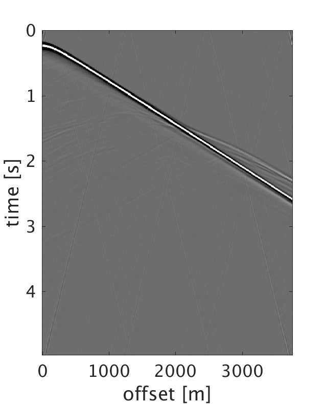
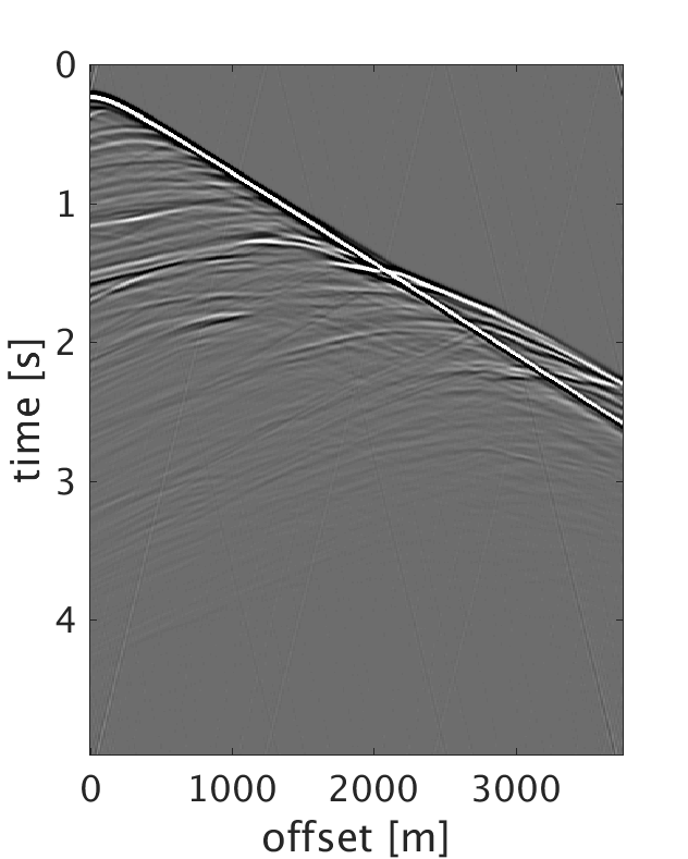
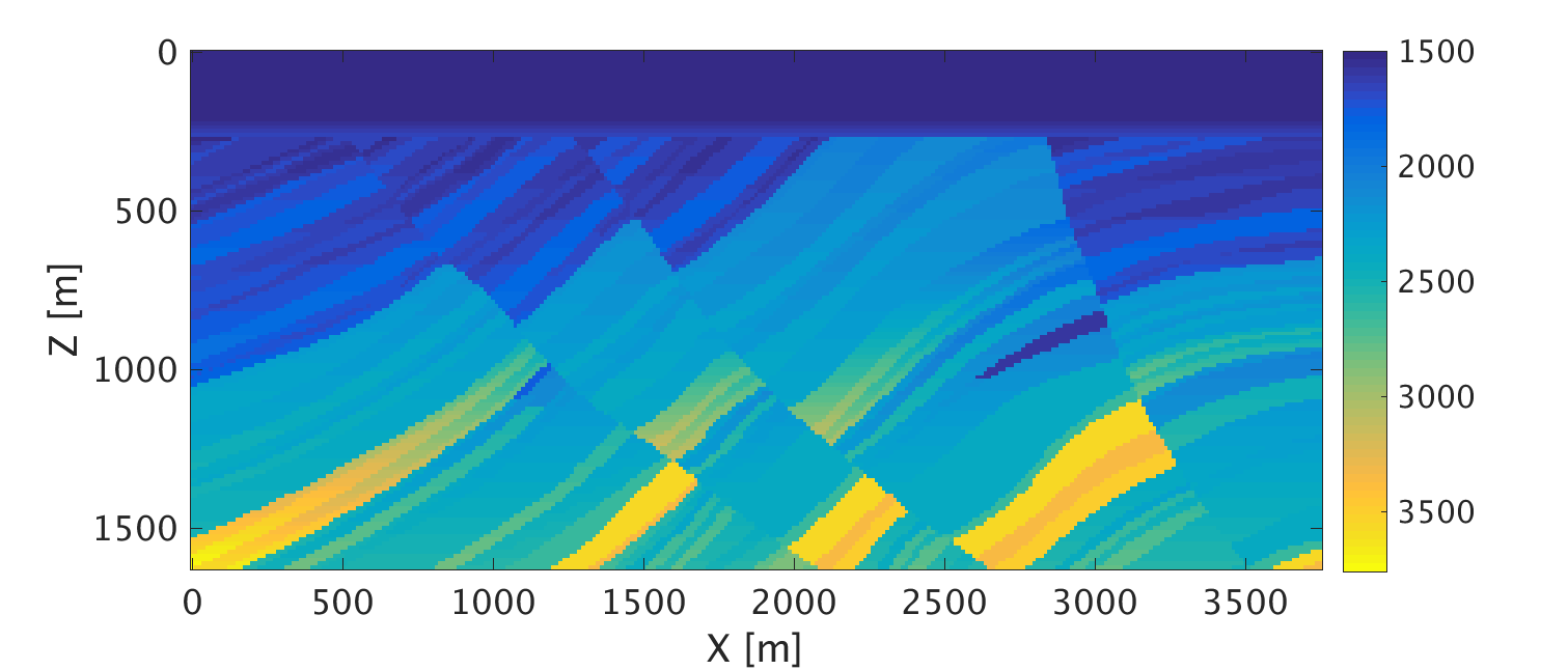
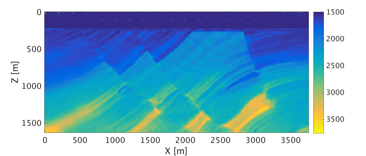
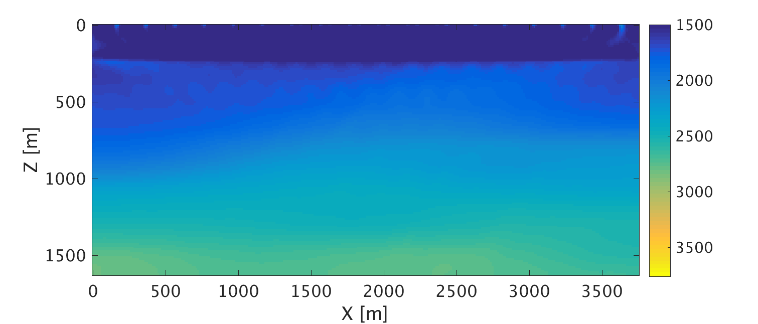
We demonstrate our proposed algorithm on non-inverse crime synthetic data using part of the Marmousi2 model, (figure 2a). We model 2D acoustic synthetic data, (figure 1a), using time-domain finite difference modeling (Thorbecke and Draganov, 2011). The acoustic data is parametrized by the P-wave velocity and density. The sources are placed near the ocean surface while the receivers are placed at the ocean bottom. The source and receiver intervals are 200m and 12.5m, respectively.

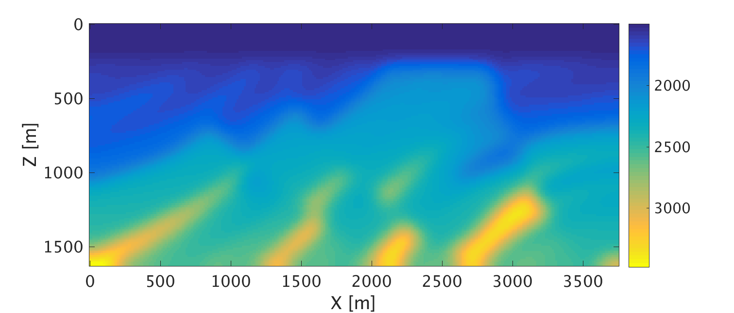
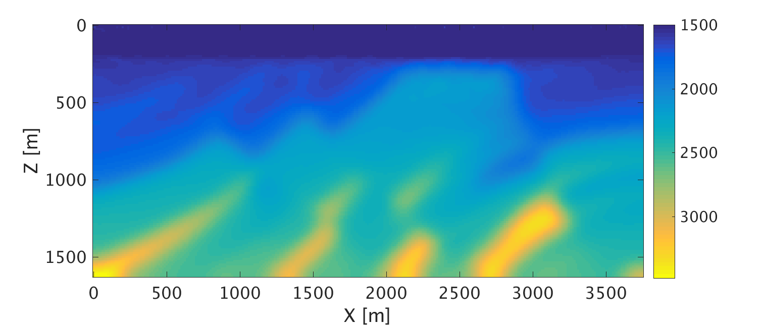
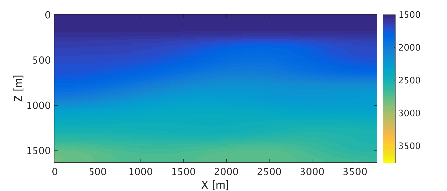
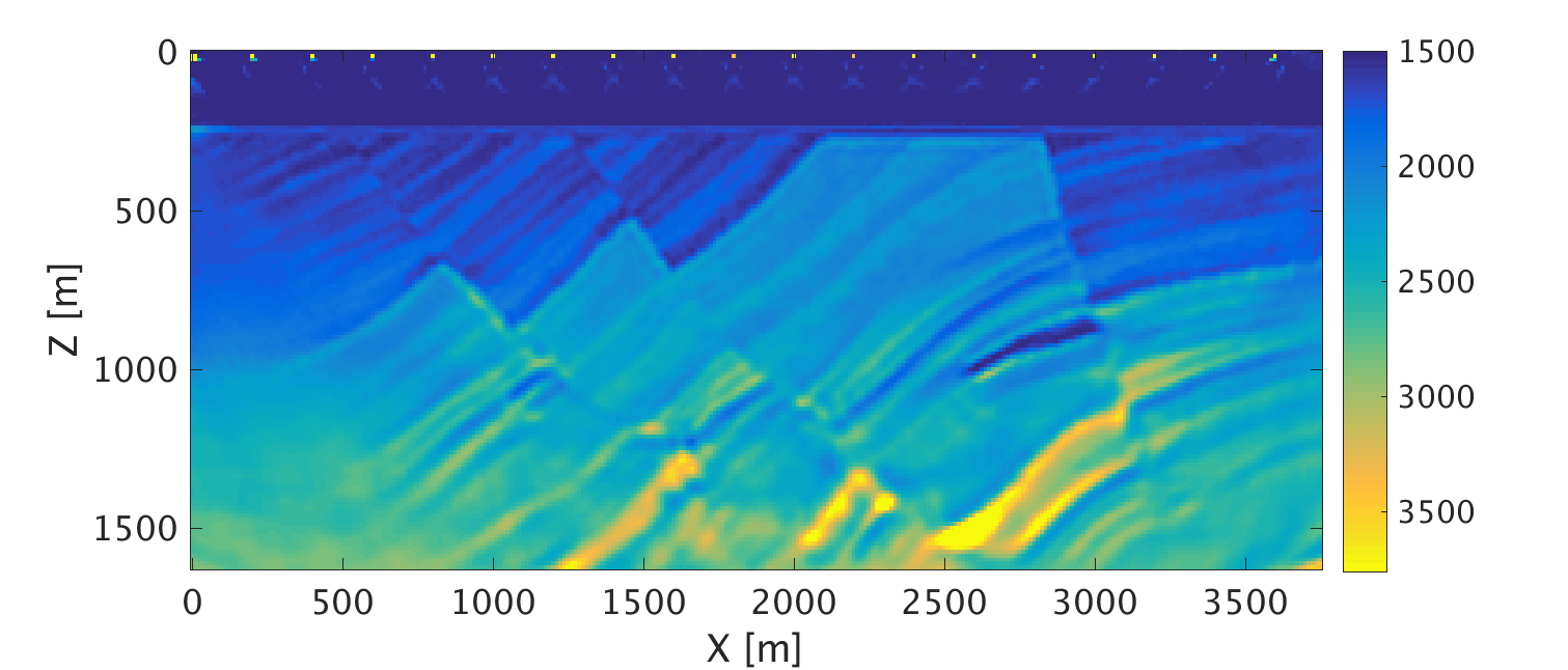
We perform P-wave velocity inversion in the time-domain using a constant-density wave-equation, see Witte et al. (2018) for more details, starting from a good initial model, (figure 2b). Figure 2c shows the result of running conventional FWI of the two-way acoustic data using the limited-memory projected quasi-Newton algorithm (Schmidt et al., 2009). We impose lower and upper bound constraints on the velocity model. Using the same initial model, (figure 2b), we run our proposed algorithm on acoustic data as follows:

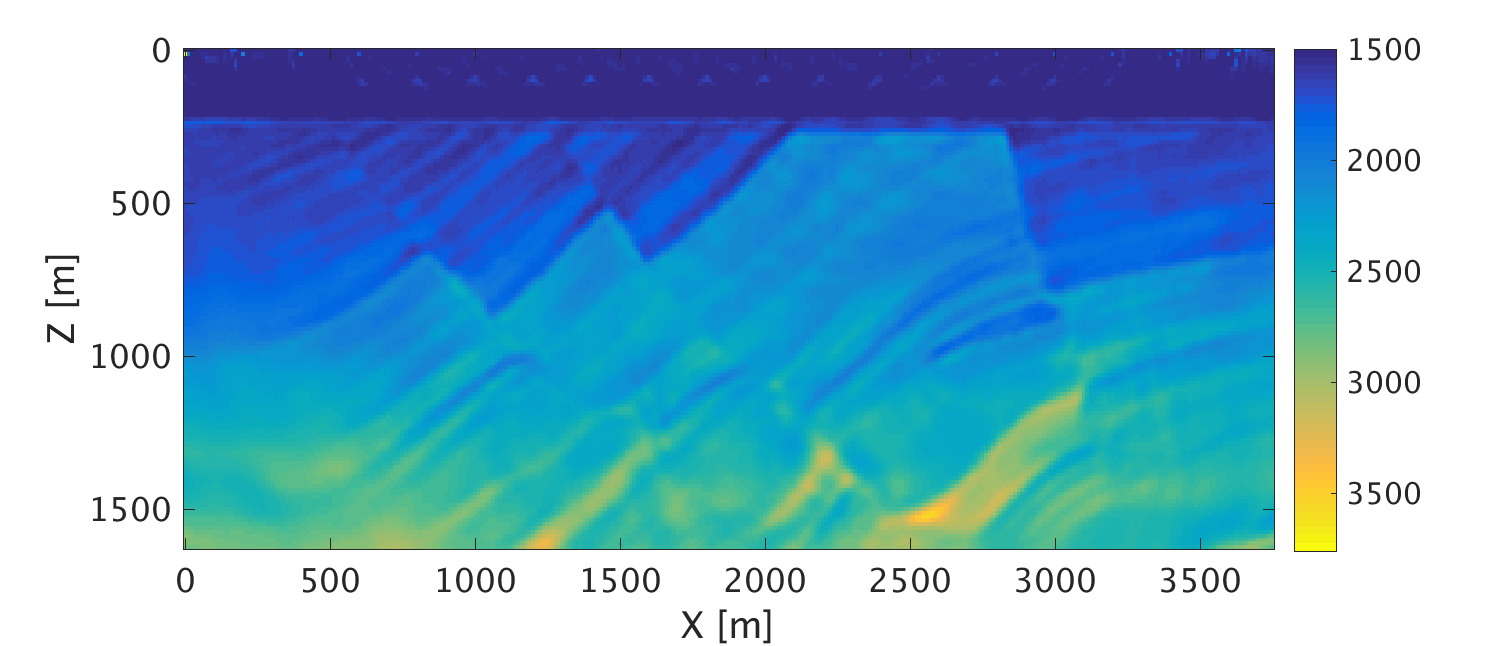
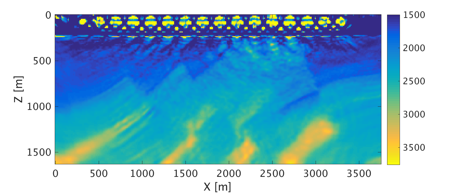
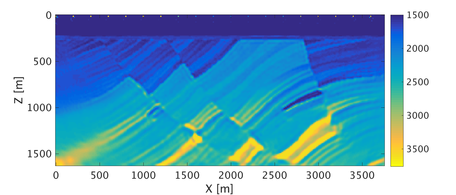
The velocity model obtained from the down-going wavefield inversion has the correct water-bottom depth compared with the initial model as well as minor model updates, (figure 2d). Compared with the model obtained from conventional acoustic FWI of the total data shown in figure 2c, the velocity model obtained from our proposed method, (figure 2e), is better resolved and the different layers and reservoirs can be easily interpreted.

When the starting model is poor, the data becomes cycle skipped, which leads to unsatisfactory velocity models. To mitigate the cycle skipping problem, we perform multi-scale inversion, (Bunks et al., 1995), starting from a poor initial velocity model, (figure 3a). We use frequencies starting from 3.5 Hz to 43 Hz. We increase the frequency bandwidth with 3 Hz after running 10 iterations at each frequency band. Comparing the multi-scale conventional FWI results, (figure 3b), with the results obtained from our proposed algorithm combined with multi-scale inversion, (figure 3d), we observe that the latter is a better velocity model with well-defined structures in the shallow and deeper parts of the model.

Another case where our proposed method is beneficial is when the sea water velocity is unknown or contain errors. The sea water velocity can change with depth because of variations in temperature and salinity. Assuming a fixed water velocity or running the inversion with a minimum water velocity of \(1500\) m/s can lead to erroneous inversion results as shown in figure 4a. We should note that in this example we constrained the minimum water velocity to the true minimum water velocity. Alternatively, we use the down-going wavefield to invert for the water velocity starting from a constant velocity model. We then incorporate this model with the good initial model used in the first example, (figure 2b), to obtain the model shown in figure 4b. This example clearly shows the importance of having accurate overburden velocity model, which we obtain by performing a relatively very small number of waveform inversion iterations using the down-going wavefields, in order to be able to obtain a satisfactory velocity model.

We demonstrated the benefits of using our proposed method on several examples to obtain improved, higher resolution and more accurate velocity models compared with conventional FWI. In terms of computational costs, it is equivalent to the computational costs of FWI as it requires less total number of iterations at least for the examples we presented. It is in our future plan to use our proposed method to estimate the S-wave velocity model from elastically decomposed data, estimate the source wavelet and investigate the cycle skipping problem.

Conclusions

We presented a method that utilizes the decomposed acoustic one-way wavefields in acoustic waveform inversion. The method simplifies the FWI problem by minimizing the difference between the decomposed one-way predicted and measured wavefields rather than using the total two-way wavefields. We implemented the method by first performing waveform inversion of the less-complicated down-going wavefields followed by waveform inversion of the more-complicated up-going wavefields using the results of the first inversion as a better initial model for the second one. We demonstrated the successful application of our proposed method on several examples using non-inverse crime acoustic synthetic data produced from the Marmousi2 model. In the case when the initial sea water velocity was inaccurate, FWI failed to provide a satisfactory model while the proposed method did not because it estimated the water velocity model first using the down-going wavefields before fitting the more complicated up-going wavefields. In all the examples, our proposed method provided improved, higher resolution and more accurate inversion results compared with conventional FWI by separately accounting for model updates from the up- and down-going wavefields.

Acknowledgements

Ali Alfaraj extends his gratitude to Saudi Aramco for sponsoring his Ph.D. studies at the University of British Columbia. This research was carried out as part of the SINBAD project with the support of the member organizations of the SINBAD Consortium.