Photoacoustic imaging with conditional priors from normalizing flows

Introduction

Photoacoustic imaging is a biomedical imaging technique based on the so-called photoacoustic effect (Xu and Wang, 2006). It leverages the interplay between optics and acoustics as a mean to circumvent the limitations of imaging modalities relying on single-type physics. Light beams generated by a pulsed laser can penetrate biological tissues by several centimeters, and are absorbed based on oxygen saturation or hemoglobin concentration. While optical absorption is in principle an ideal parameter for medical imaging (e.g., with respect to the detection of cancerous tissue), strong scattering imposes important limitations in its imaging resolution. Ultrasonics, on the other hand, can theoretically provide resolution of medical diagnostic value, but produce images of mechanical properties whose contrasts are not sensitive for detecting early stage tumors. In photoacoustics, optical and acoustic effects are combined to gain the best of both worlds. Under conditions of thermal and stress confinement, where the light pulse duration is negligible with respect to the heat diffusion and stress propagation time scales, thermal energy can efficiently build up in biological tissues, which in turn undergo thermal expansion and effectively act as a spatially distributed acoustic source. In photoacoustic imaging, the actual object of interest is the induced source, as it is directly related to optical absorption and can be recovered with a relatively higher resolution than pure optical imaging, based on the acquired ultrasonic data.

Photoacoustic imaging boils down to an initial value problem. The pressure field \(p\), function of space and time, obeys the acoustic wave equation: \[ \begin{equation} \begin{aligned} \left\{ \begin{array}{rcl} c^{-2}\partial_{tt}p-\Delta p & = &0,\\ \partial_t p|_{t=0} & = & 0,\\ p|_{t=0} & = & p_0. \end{array} \right. \end{aligned} \label{eq:wave-equation} \end{equation} \] We assume that the velocity parameter \(c\) is a positive constant (though this could be easily extended to the inhomogeneous case). We are interested in retrieving the initial pressure distribution \(p_0\) from acoustic data. However, due to the intrinsic limitations of optics, the viable imaging depth for human tissue ranges around 1-4 cm, so that the receiver geometry has typically a one-sided view of the object (as for planar sensors, Jathoul et al., 2015). This restricted view poses serious challenges for photoacoustic imaging.

Due to measurement incompleteness, one has to resort to prior information. In a Bayesian setting, we posit a data likelihood \(\mathbf{d}=A\mathbf{x}+\pmb{\varepsilon}\), where the Gaussian white noise \(\pmb{\varepsilon}\) is independent from \(\mathbf{x}\), which represents the initial distribution value \(p_0\) appearing in equation \(\eqref{eq:wave-equation}\). The linear operator \(A\) comprises the solution of the equation \(\eqref{eq:wave-equation}\) followed by the restriction to the receiver position. The prior information is encapsulated by a probability density \(p_{\mathrm{prior}}\). The solution is estimated by solving the problem: \[ \begin{equation} \min_{\mathbf{x}}\dfrac{1}{2}\left\lVert A\mathbf{x}-\mathbf{d}\right\rVert^2-\lambda\log p_{\mathrm{prior}}(\mathbf{x}), \label{eq:minimization} \end{equation} \] for a given weighting parameter \(\lambda\), to be properly tuned. For example, the compressed sensing paradigm enforces sparsity of the unknown in some transformed domain via \(\ell^1\)-norm regularization. This class of “hand-crafted” priors are well studied from a theoretical point of view (Candes et al., 2006), but they typically do not take advantage of domain-specific knowledge of the problem.

In recent years, many applications of deep learning to linear inverse problems have dealt with priors implicitly defined by neural networks, e.g. by pre-training a generative network on a collection of candidate solutions (Bora et al., 2017) or without training by directly exploiting the network inductive bias that favors natural-looking images (Ulyanov et al., 2018). Our proposal consists of a deep prior solution to photoacoustic imaging, similarly to Bora et al. (2017), where the generative model is now trained on joint pairs of photoacoustic sources and associated measurements. The network is structured as a conditional normalizing flow (Ardizzone et al., 2019; Winkler et al., 2019), so that it is able to generate samples from the posterior distribution of \(\mathbf{x}\) given data \(\mathbf{y}\). For out-of-distribution data \(\mathbf{y}\), however, the learned posterior distribution does not adequately represent the analytical posterior. We then resort to the physics-based formulation in equation \(\eqref{eq:minimization}\) in combination with the learned conditional prior to compute the maximum a posteriori solution (MAP). Our approach takes advantage of the favorable trade-off between the representation error and overfit for invertible networks when compared to other generative models (Asim et al., 2020; Kelkar et al., 2021).

Related work

The regularization scheme described in this paper follows the deep prior literature originally spun from the work of Bora et al. (2017), which consists in reparameterizing the inverse problem unknowns by the input of a pre-trained generator. A closely related method is the deep image prior of Ulyanov et al. (2018), which aims to counteract the potential representation error that might affect a pre-trained network. Contrary to Bora et al. (2017), the unknowns are now the network parameters, randomly initialized, while the input remains fixed. This method must resort to early stopping strategy to avoid overfit and only relies on the regularization effect of the network inductive bias. The complementary strenghts of these two approaches can be combined in a hybrid scheme, e.g. by using image-adaptive priors (Hussein et al., 2020). Our proposal is similar to the deep prior application to magnetic resonance imaging discussed in Kelkar et al. (2021), which uses invertible networks and further regularization of the latent-space variables. The advantages of using normalizing flows in the deep prior context were originally advocated by Asim et al. (2020). We extend the normalizing flow approach by using conditional architectures, as described in Ardizzone et al. (2019) and Winkler et al. (2019). Normalizing flows have been subject to a great deal of research, we refer to Kobyzev et al. (2020) and Papamakarios et al. (2019) for general overviews. The network architecture analyzed in this paper is HINT, discussed in Ardizzone et al. (2018) (and later generalized to the conditional setting in Ardizzone et al. (2019)). An application of conditional normalizing flows in variational inference was recently discussed in Siahkoohi et al. (2021).

Method

The proposed method aims at regularizing the inverse problem in equation \(\eqref{eq:minimization}\) with a learned prior. The first stage of the algorithm consists of training a generator given access to a dataset of joint pairs \(\mathbf{x},\mathbf{y}\sim p_{X,Y}(\mathbf{x},\mathbf{y})\), where \(\mathbf{y}=A^T\mathbf{d}\) is time-reversed data (referred to as the adjoint solution). We train a normalizing flow \(f_{\pmb{\theta}}:X\times Y\to Z_x\times Z_y\) by minimizing the Kullback-Leibler divergence between the target density \(p_{X,Y}\) and the pull-back of the standard Gaussian distribution defined on the latent space \(Z_x\times Z_y\) via \(f_{\pmb{\theta}}\) (Kobyzev et al., 2020; Papamakarios et al., 2019): \[ \begin{equation} \min_{\pmb{\theta}}\mathrm{KL}(p_{X,Y}\lVert p_{\pmb{\theta}})=\mathbb{E}_{\mathbf{x},\mathbf{y}\sim p_{X,Y}(\mathbf{x},\mathbf{y})}\dfrac{1}{2}\left\lVert f_{\pmb{\theta}}(\mathbf{x},\mathbf{y})\right\rVert^2-\log|\det\mathrm{J}_{f_{\pmb{\theta}}}(\mathbf{x},\mathbf{y})|. \label{eq:KLmin} \end{equation} \] Here, \(\mathrm{J}_{f_{\pmb{\theta}}}\) denotes the Jacobian of \(f_{\pmb{\theta}}\) with respect to the input. Following Ardizzone et al. (2019), we impose a triangular structure on the normalizing flow, e.g. \(f_{\pmb{\theta}}(\mathbf{x},\mathbf{y})=(f^{z_x}_{\pmb{\theta}}(\mathbf{x},\mathbf{y}),f^{z_y}_{\pmb{\theta}}(\mathbf{y}))\). We choose the conditional architecture of the HINT invertible network, whose original (non-conditional) form was proposed in Ardizzone et al. (2018). After an ideal optimization of equation \(\eqref{eq:KLmin}\), sampling from the posterior distribution \(\mathbf{x}\sim p_{X|Y}(\mathbf{x}|\mathbf{y})\) is equivalent to computing the latent data code \(\mathbf{z}_y=f^{z_y}_{\pmb{\theta}}(\mathbf{y})\) and evaluating \(f^{-1}_{\pmb{\theta}}(\mathbf{z}_x,\mathbf{z}_y)\) for random \(\mathbf{z}_x\)’s. This first phase does not require repeated evaluation of the physical model \(A\) appearing in equation \(\eqref{eq:minimization}\), which helps in relieving the computational burden given by solving partial differential equations at scale.

When faced with out-of-distribution data, we can reasonably assume that the results previously obtained are not as reliable as for in-distribution data. The second stage of the proposed method then relies on the physics model in equation \(\eqref{eq:minimization}\) and uses the pre-trained generator as an implicit deep prior. Formally, we end up solving the problem: \[ \begin{equation} \min_{\mathbf{z}_x}\dfrac{1}{2}\left\lVert A\,f^{-1}_{\pmb{\theta}}(\mathbf{z}_x,\mathbf{z}_y)-\mathbf{d}\right\rVert^2+\dfrac{\phantom{^2}\lambda^2}{2}\left\lVert\mathbf{z}_x\right\rVert^2,\quad\mathbf{z}_y=f^{z_y}_{\pmb{\theta}}(A^T\mathbf{d}). \label{eq:deepprior} \end{equation} \] Note that the minimization is carried over the latent variables related to the unknowns \(\mathbf{x}\). The computational effort to evaluate \(A\) and its adjoint is managenable when single data \(\mathbf{d}\) is considered.

Results

The results related to the training of the generative model are collected in Figure 1. The training set consists of images of blood vessel systems \(\mathbf{x}\) and time-reversed data \(\mathbf{y}=A^T\mathbf{d}\) measured at the receiver location located on top of the image (Hauptmann and Cox, 2020). The measurements are generated synthetically by solving the wave equation and adding Gaussian white noise. We qualitatively compare samples drawn from the learned posterior distribution for in- and out-of-distribution data.

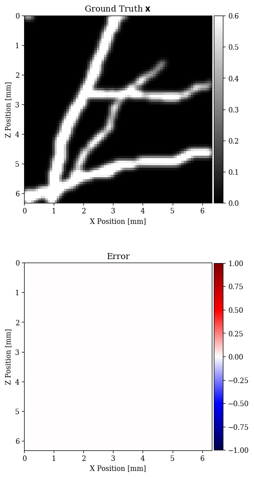
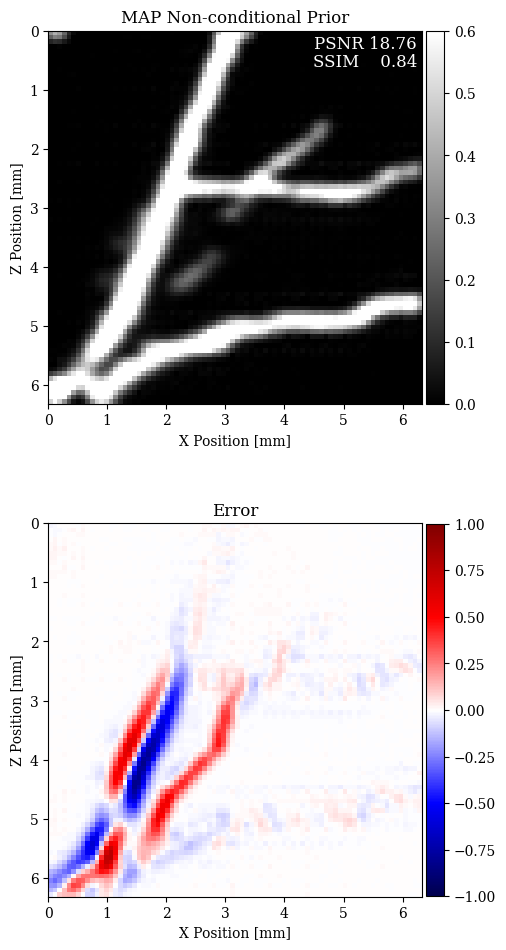
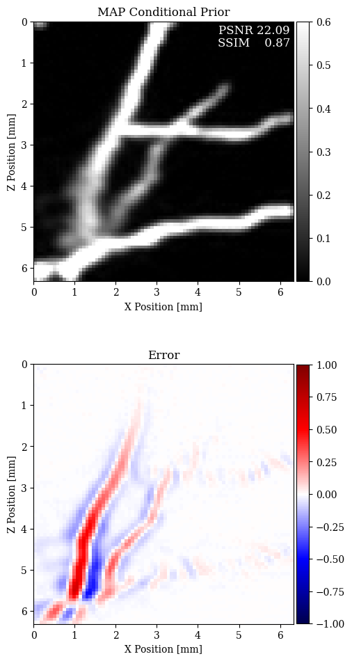
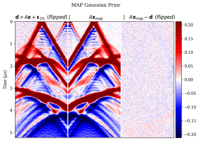
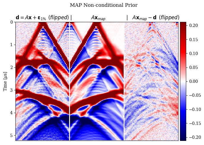
In Figure 2, we compare the reconstruction results for out-of-distribution data by solving the problem in equation \(\eqref{eq:minimization}\) with different choices for the prior. In particular, we consider a non-informative Gaussian prior and learned priors trained on a dataset of samples \(\mathbf{x}\)’s and joint pairs \(\mathbf{x},\mathbf{y}\)’s (our proposal). A qualitative inspection and quality metrics indicate superior results for the conditional prior approach. Further comparison of the results regarding data fit is shown in Figure 3.

Discussion and conclusions

In limited-view photoacoustic imaging, the resolution of deep near-vertical structures in a blood vessel system is a fundamental challenge due to the relatively weak imprint on the measurements. Note that similar issues are common for other wave-equation-based imaging applications such as geophysical prospecting (Tarantola, 2005). Conventional regularization methods based on sparsity in some transformed domain are typically too generic and practically unable to fill the sensitivity gap. A straightforward alternative is to use problem-specific information.

We proposed a regularization scheme for photoacoustic imaging that employs deep priors learned in an offline phase. The generative model is trained on a dataset containing pairs of candidate solutions and associated measurements, the goal is to learn the posterior distribution of the solution given some data. The primary scope of this work is to compare the regularization effect of conditional deep priors with “marginal” deep priors proposed in the recent past for many imaging applications. With “marginal” priors, we refer to generative models trained on the marginal distribution of the unknowns (e.g. without considering the associated data).

The results presented in this paper suggest that the MAP estimate based on conditional deep priors is potentially able to recover the vertical features of a blood vessel image. Our results also show that the marginal deep prior is more prone to misplace features, for both in- and out-of-distribution data.

In our view, learned prior regularization can be beneficial for highly ill-posed problems such as limited-view photoacoustic imaging. In order to avoid misleading reconstruction affected by “hallucinations”, however, we must further assess the strong bias imposed by this type of learned priors.

Data and software

The dataset used in this work is a derivative of the ELCAP lung dataset prepared by Hauptmann and Cox (2020). The results presented here uses a Julia implementation of invertible network architectures: InvertibleNetworks.jl (P. Witte et al., 2020).