Wave-equation based inversion with amortized variational Bayesian inference

Introduction

An inverse problem involves reliably estimating an unknown quantity from noisy indirect observations. This problem is commonly solved using optimization techniques to minimize the difference between predicted and observed data. Solely minimizing the data misfit negatively impacts the quality of the obtained solution due to noise in the data, modeling errors, and a nontrivial null-space of the forward operator (Tarantola, 2005). To prevent this, it is crucial to capture and incorporate prior knowledge into the inverse problem (Tarantola, 2005), e.g., Gaussian or Laplace distribution priors (Malinverno and Briggs, 2004; Martin et al., 2012; F. J. Herrmann and Li, 2012). While theoretically understood, these type of priors may lead to undesirable biases in the outcome of inversion.

The purpose of our contribution is to address this challenge by utilizing a formulation that exploits a data-driven conditional prior. To achieve this, following Orozco et al. (2021), we train a conditional normalizing flow (NF, Kruse et al., 2021) to capture the conditional distribution of the unknown, given data, i.e., the posterior distribution. The training involves minimizing an amortized variational inference objective (Jordan et al., 1999; Siahkoohi et al., 2021b; Siahkoohi and Herrmann, 2021; Kruse et al., 2021; Kovachki et al., 2021) using existing training pairs in the form of low-fidelity data and model pairs. After training, we are able to capture the low-fidelity posterior distribution for previously unseen seismic data. We use the this network to reparameterize the unknown in an inversion scheme, involving physics-guided data misfit and a Gaussian prior on the NF latent variable. Due to the inherent invertibility of NFs, they can represent any model in the unknown space, which allows them to be be used as priors when dealing with out-of-distribution data (Asim et al., 2020; Orozco et al., 2021).

There are three key advantages to our proposed method: (1) Data-driven priors make use of available data, such as high-resolution seismic images to capture prior knowledge about the Earth’s subsurface; (2) The use of a conditional prior favors solutions that are consistent with the data, which provides more specific knowledge about the unknown; (3) With the help of our formulation, we combine data-driven priors with conventional physics-based inversion methods, which offers the advantages of data-driven priors without relying solely on them as a black box.

In the following sections, we discuss conditional NFs, trained using an amortized variational inference procedure. Next, we present an inversion scheme for seismic imaging that incorporates conditional priors. We conclude by demonstrating this technique on a realistic seismic imaging problem involving noisy and out-of-distribution data.

Amortized variational inference

The problem setup entails applying variational inference (Jordan et al., 1999) to approximate the posterior distribution (Tarantola, 2005) associated with the inverse problem \(\B{y} = F (\B{x}) + \boldsymbol{\epsilon}\), where \(\B{y} \in Y\) represents the observed data, \(\B{x} \in X\) unknown model, \(\boldsymbol{\epsilon}\) possibly non-Gaussian noise, and \(F: X \rightarrow Y\) the possibly nonlinear forward operator. In the context of amortized variational inference (Kruse et al., 2021), we wish to approximate the posterior distribution associated with this inverse problem for previously unseen data. This method has computational advantages as it does not require solving an additional instance of variational inference for new data. In this work, we choose NFs (Rezende and Mohamed, 2015) that due to their invertibility (up to numerical precision) can be used to approximate a target distribution, of which we have only samples. NFs can be adapted to sample from the conditional distribution \(p(\B{x} \mid \B{y})\) by using a block-triangular construction (Marzouk et al., 2016), \(T_{\R{w}} (\B{y}, \B{x}) =(T_{\R{w}_1} (\B{y}), T_{\R{w}_2} (\B{y}, \B{x}))\) with \(\B{w} = (\B{w}_1, \B{w}_2)\). The conditional NF \(T_{\R{w}} : Y \times X \rightarrow Z \times Z\), which takes as input data and model pairs \((\B{y}, \B{x})\), aims to yield two normally distributed outputs in the latent space \(Z \times Z\). Training objective is based on minimizing the Kullback-Leibler divergence between the NF output distribution and the Gaussian latent distribution (Kruse et al., 2021): \[ \begin{equation} \mathop{\rm arg\,min}_{\B{w}}\, \frac{1}{n} \sum_{i=1}^n \Bigg[ \frac{1}{2}\big\| T_{\R{w}} (\B{y}^{(i)}, \B{x}^{(i)}) \big\|^2_2 - \log \Big | \det \nabla_{(\R{y}, \R{x})} T_{\R{w}} (\B{y}^{(i)}, \B{x}^{(i)}) \Big |\Bigg]. \label{NF-training-cond} \end{equation} \] In the above objective, the \(\ell_2\)-norm follows from a Gaussian assumption on the latent variables and the second term is a regularization term that avoids \(T_{\R{w}}\) from converging to trivial solutions—e.g., \(T_{\R{w}} := \B{0}\). Computing \(\det \nabla_{(\R{y}, \R{x})} T_{\R{w}} (\B{y}, \B{x})\) and its gradient adds almost no extra cost because of the particular design of invertible networks (Dinh et al., 2016). Following training, we can obtain samples from conditional distribution \(p(\B{x} \mid \B{y})\) via \(T_{\R{w}_2}^{-1} \big( T_{\R{w}_1} (\B{y}), \B{z} \big) \sim p(\B{x} \mid \B{y}), \ \B{z} \sim p_{\R{z}}(\B{z})\) (Marzouk et al., 2016; Kruse et al., 2021). This amounts to feeding the latent code associated with observed data, i.e., \(T_{\R{w}_1} (\B{y})\), and Gaussian samples \(\B{z} \sim p_{\R{z}}(\B{z})\) into the inverse network, \(T_{\R{w}_2}^{-1}\). These samples may be used for Bayesian inference if we have an ideal training dataset (F. J. Herrmann et al., 2019; Siahkoohi and Herrmann, 2021; Kumar et al., 2021; Kothari et al., 2021). However, such an assumption is rarely correct in geophysical applications due to Earth’s strong heterogeneity (Siahkoohi et al., 2019, 2021a; Sun and Demanet, 2020), which highlights the importance of devising formulations that are robust to changes in data distribution during inference.

Seismic imaging with data-driven conditional priors

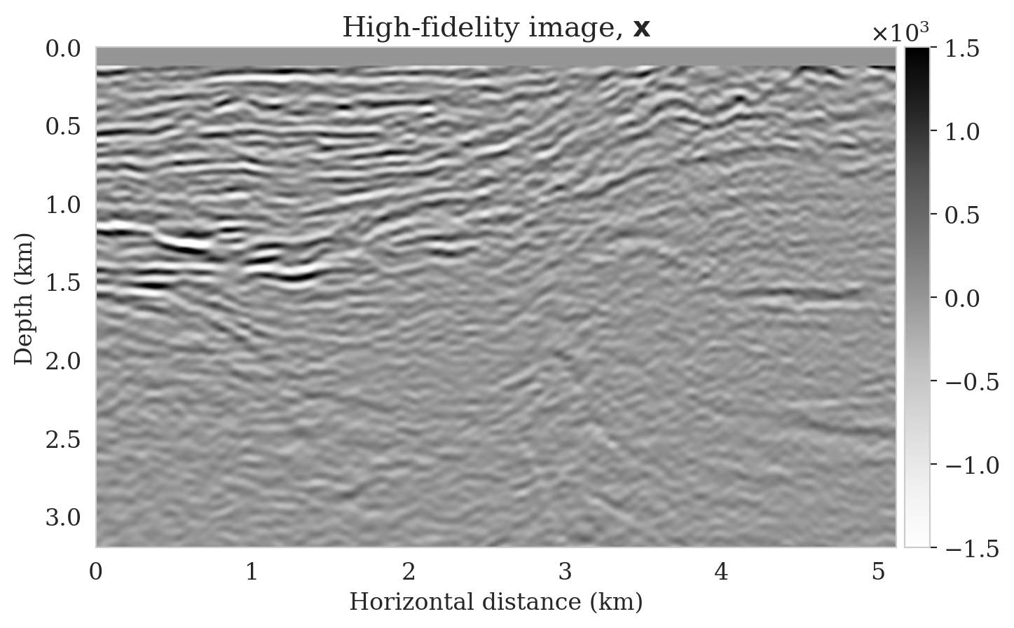
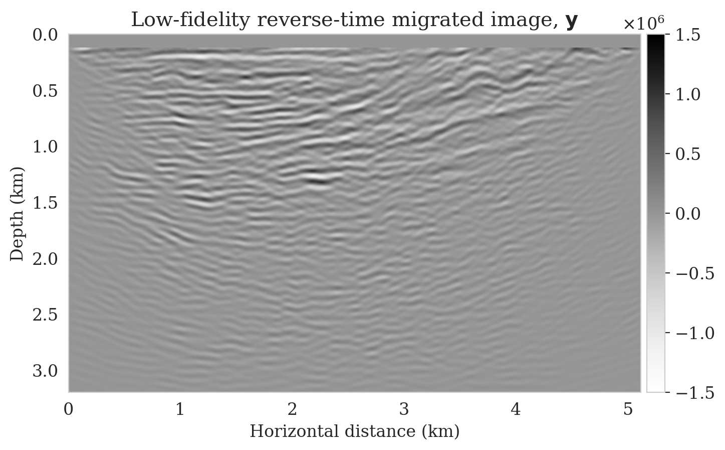
Using multiple processed shot records, \(\left \{\B{d}_{i}\right \}_{i=1}^{n_s}\), seismic imaging aims to estimate the short-wavelength component of the Earth’s subsurface squared-slowness model, denoted by \(\delta \B{m}\). The linearized Born scattering operator \(\B{J}(\B{m}_0, \B{q}_i)\) relates the unknown seismic image \(\delta \B{m}^{\ast}\), to data, the \(i\text{th}\) source signature, \(\B{q}_{i}\), and the background squared-slowness model \(\B{m}_0\). This relation can be written as \[ \begin{equation} \B{d}_i = \B{J}(\B{m}_0, \B{q}_i) \delta \B{m}^{\ast} + \boldsymbol{\epsilon}_i, \quad \boldsymbol{\epsilon}_i \sim \mathrm{N} (\B{0}, \sigma^2 \B{I}). \label{linear-fwd-op} \end{equation} \] Noise is denoted by \(\boldsymbol{\epsilon}_i\) and represents measurement noise and linearization errors, which for simplicity is assumed to be distributed according to a zero-centered Gaussian distribution with known covariance \(\sigma^2 \B{I}\). We train a NF on pairs of low- and high-fidelity seismic images via the amortized variational inference objective by choosing \(\B{x}\) to represent high-fidelity migrated images and \(\B{y} := \delta\B{m}_{\text{RTM}}\) corresponding to low-fidelity reverse-time migrated images obtained by the process of demigration, followed by adding noise and migration. After training, the conditional NF captures the low-fidelity seismic imaging posterior distribution. In order to obtain a high-fidelity seismic image maximum a posteriori (MAP) estimate, we propose to reparameterize \(\delta \B{m}\) vis the pretrained NF and solve the optimization problem \[ \begin{equation} \widehat{\B{z}} = \argmin_{\B{z}}\, \frac{1}{2 \sigma^2} \Bigg[ \sum_{i=1}^{n_s}\big \| \B{d}_i- \B{J}(\B{m}_0, \B{q}_i) T_{\R{w}_2}^{-1} \big( T_{\R{w}_1} (\delta\B{m}_{\text{RTM}}), \B{z} \big) \big \|_2^2 \Bigg] + \frac{1}{2} \big \| \B{z} \big \|_2^2, \label{imaging-opt-nf} \end{equation} \] followed by mapping \(\delta\B{m}_{\text{MAP}} := T_{\R{w}_2}^{-1} \big( T_{\R{w}_1} (\delta\B{m}_{\text{RTM}}), \widehat{\B{z}} \big)\). We initialize optimization problem \(\ref{imaging-opt-nf}\) with \(\B{z}_0 = \B{0}\). This initialization and a Gaussian prior on \(\B{z}\) regularize the inversion by favoring solutions that are likely samples of the low-fidelity posterior distribution (Asim et al., 2020). NFs’ inherent invertibility allows them to represent any image \(\delta \B{m}\) in the solution space. This limits the potentially negative bias of the conditional prior in domains where access to high-fidelity training data is limited. We demonstrate this through a numerical experiment in the next section.

Numerical experiments

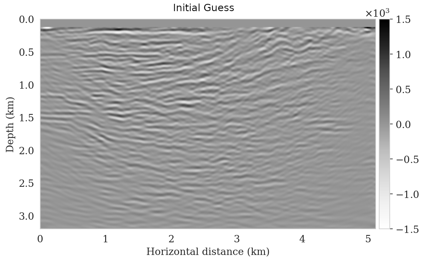
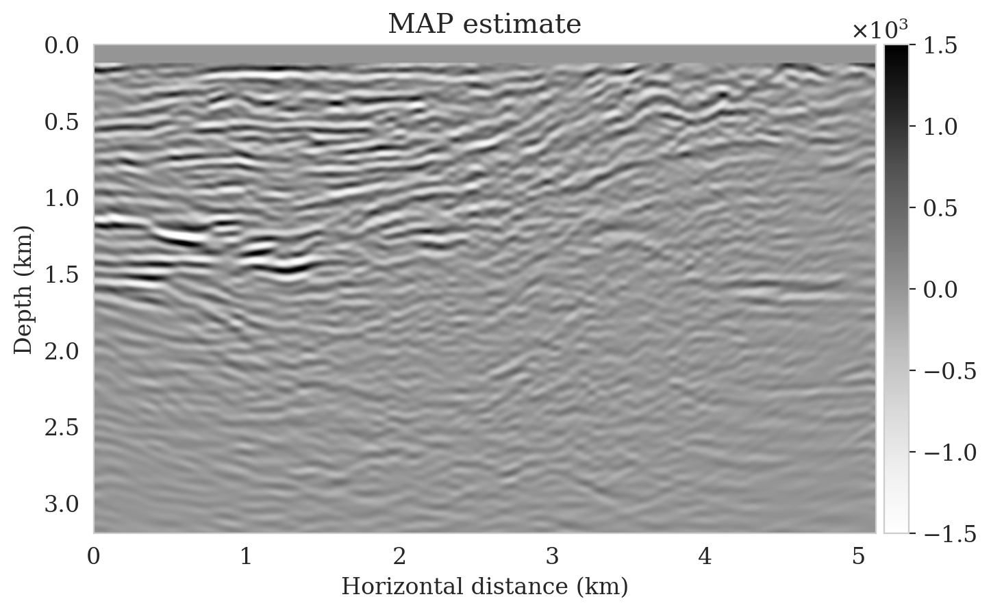
We propose a realistic example in which we create \(4750\) 2D training pairs of low- and high-fidelity seismic images, which the latter are \(3075\, \mathrm{m} \times 5120\, \mathrm{m}\) sections extracted from the shallow part of Parihaka (WesternGeco., 2012) prestrack Kirchhoff migration dataset. The low-fidelity images are obtain by migrating noisy synthetic data obtained from the high-fidelity images according to Equation \(\ref{linear-fwd-op}\). The acquisition geometry involves \(102\) shot records, \(204\) fixed receivers, Ricker wavelet with a central frequency of \(30\, \mathrm{Hz}\), and band-limited noise. We augment a \(125\, \mathrm{m}\) water column on top of these models to limit the near source imaging artifacts. We train \(T_{\R{w}}\) according to the objective function in Equation \(\ref{NF-training-cond}\) with the Adam optimization algorithm (Kingma and Ba, 2014). In order to evaluate the effectiveness of our inversion scheme when applied to out-of-distribution data, we select a 2D section from the deeper portions of the Parihaka dataset (see Figure 1a). As compared to training images, this image includes more noncontinuous reflectors, due to low signal-to-noise ratio in the deeper parts of the Parihaka dataset. We simulated linearized data with the same acquisition geometry described above to obtain a low-fidelity image (Figure 1b). We solve optimization problem \(\ref{imaging-opt-nf}\) for \(5\) passes over the shot records, i.e., approximately the same cost as 5 reverse-time migrations. Figure 1c shows the initial guess of the optimization, i.e., \(T_{\R{w}_2}^{-1} \big( T_{\R{w}_1} (\delta\B{m}_{\text{RTM}}), \B{z}_0 \big)\). We can see that this image is not correctly recovering the reflectors, however, it can be considered a better starting guess than the reverse-time migrated image (Figure 1b) due to corrected amplitudes. Finally, Figure 1d shows the MAP estimate, obtained via solving the optimization problem \(\ref{imaging-opt-nf}\), which successfully reconstructs most of the reflectors with limited artifacts.

Our example uses JUDI (P. A. Witte et al., 2019) to construct wave-equation solvers, which utilizes Devito (Luporini et al., 2018; M. Louboutin et al., 2019) as a highly optimized finite difference solver under the hood. The network architectures are implemented using InvertibleNetworks.jl (Witte et al., 2021), a memory-efficient framework for training invertible nets in Julia. Sample code to reproduce the results is provided on GitHub.

Conclusions

Considering the Earth’s strong heterogeneity, designing regularization schemes to incorporate prior knowledge for solving ill-posed geophysical inverse problems is challenging. To address this challenge, we proposed a regularization scheme that takes advantage of existing data in the form of low- and high-fidelity seismic images to train a conditional normalizing flow (NF). This conditional NF approximates the imaging posterior distribution for previously unseen data. In order to minimize the impact of data distribution shifts during inference, we reparameterized the unknown image with the conditional NF and inverted for a Gaussian latent variable that fits the data. The resulting maximum a posteriori estimate takes advantage of the data-driven conditional prior while remaining bound to data and physics. Using numerical experiments, we demonstrated that this approach yields seismic images with limited imaging artifacts in the absence of high-fidelity training data. Further research on quantifying the uncertainty through this regularization technique is required.

Acknowledgment

This research was carried out with the support of Georgia Research Alliance and partners of the ML4Seismic Center.