Seismic data reconstruction with Generative Adversarial Networks

Ali Siahkoohi\(^{1*}\), Rajiv Kumar\(^{1,2}\) and Felix J. Herrmann\(^2\)
\(^1\)Seismic Laboratory for Imaging and Modeling (SLIM), The University of British Columbia,
\(^2\)Georgia Institute of Technology

Introduction

Densely regularly sampled seismic data yields higher resolution images using current imaging techniques. Sampling wavefields at Nyquist-rate is expensive and time consuming given the large dimensionality and size of seismic data volumes. In addition, fully-sampled data recovered from equally-spaced under-sampled data may suffer from residual aliasing artifacts. Compressed Sensing methods recover the fully-sampled data form highly incomplete sets of linear measurements using sparsity promoting iterative solvers. The underlying assumption in sparse signal recovery is that data with missing samples is less sparse than the fully-sampled data, in some transform domain. This requires a randomized sampling scheme to break the sparsity in the transform domain. There has been efforts to randomize the acquisition of seismic data (Wason and Herrmann, 2013) and it requires special acquisition design. This means vintage data that already has been shot does not satisfy the underlying assumption in sparse signal recovery.

We can categorize the previous methods for seismic data reconstruction as follows. Some methods use a transform domain in which the fully-sampled data is sparse. They recover the signal using sparsity-promoting methods (M. D. Sacchi et al., 1998; Herrmann and Hennenfent, 2008; Hauser and Ma, 2012). The redundancy of seismic data can also be exploited when data is reshaped into a matrix. Oropeza and Sacchi (2011) and Kumar et al. (2013) used rank minimization techniques to reconstruct the missing values. Da Silva and Herrmann (2014) and Kreimer et al. (2013) used tensor completion methods to reconstruct seismic data. And finally dictionary learning methods have also been utilized to recover missing values in seismic data (L. Zhu et al., 2017; Yarman et al., 2017).

The above mentioned methods, rely on some perhaps too simplifying assumptions on data by formulating linear mathematical models that explain the data either as a superposition of prototype waveforms from a fixed or learned dictionary or in terms of a matrix factorizations. Although data-adaptive schemes such as dictionary learning and matrix factorizations have been successful, these approaches because of their linearity may fail to capture information hidden in (seismic) data. By giving up linearity and using adaptive nonlinear models, combined with insights from game theory, we arrive at a new formulation for missing-trace interpolation where the signal model is no longer linear —i.e., the data is no longer considered as a superposition of basic elements.

While there is an abundance of nonlinear signal models, not in the least ones that are defined in terms of the wave equation itself that is nonlinear in the medium properties, we propose the use of deep convolutional neural networks (CNNs, Krizhevsky et al., 2012) and in particular the state-of-the-art Generative Adversarial Networks (GANs, Goodfellow et al., 2014). GANs are able to learn to sample from high dimensional complex probability distributions without making strong assumptions on the data.

Nonlinear models outperform linear approximations to the complex nonlinear real-world models because they can capture the nonlinearities of observed data. On the other hand, the formulation of an appropriate nonlinear function to model a particular phenomena requires knowledge of underlying data generation process that can be unknown. In principle, wave equations are the underlying ideal nonlinear data generation process for seismic data provided these equations capture the full wave physics, which is not always the case for various reasons. Based on universal approximation theory (Csáji, 2001), neural networks can approximate any continuous function under some mild assumptions. This motivates us to use neural networks, in particular, GANs with a probabilistic approach, to implicitly model the complex nonlinear probability distribution of the data, rather than the nonlinear physical model itself. By deploying this model and with access to training dataset, we hope to outperform current methods for large percentages of traces missing and without imposing constraints on the type of (random) sampling.

Generative Adversarial Networks

Suppose we have a set of samples \(S_X = \left \{ \mathbf{x}_i \right \}_{i=1}^{N}\) drawn from an initial distribution \(p_X (\mathbf{x})\) and a set of samples \(S_Y = \left \{ \mathbf{y}_i \right \}_{i=1}^{N}\) drawn from a target distribution \(p_Y (\mathbf{y})\), where \(N\) is the number of samples in each set. The goal is to learn a mapping \(\ \mathcal{G}: X \rightarrow Y\). In other words, not only map \(S_X\) to \(S_Y\), but also map all the samples from \(p_X (\mathbf{x})\) to samples from \(p_Y (\mathbf{y})\). GANs consist of two deep CNNs, namely the generator \((\mathcal{G})\), and the discriminator \((\mathcal{D})\), which can achieve the goal of training the generative network via an adversarial game. The game is described as follows:\(\ \mathcal{D}: \mathbb{R}^{m \times n} \rightarrow [0, 1]\) estimates the probability that a sample came from the \(p_Y (\mathbf{y})\) rather than from the of output of \(\mathcal{G}\). The generator \(\mathcal{G}\) maps \(p_X (\mathbf{x})\) to \(p_Y (\mathbf{y})\) such that it’s output is difficult for \(\mathcal{D}\) to distinguish from the samples in \(p_Y (\mathbf{y})\). Let \(\theta^{(\mathcal{G})}\) and \(\theta^{(\mathcal{D})}\) be the set of parameters for networks \(\mathcal{G}\) and \(\mathcal{D}\), respectively. We can describe the GAN objective as a combination of the generator and the discriminator objective functions as follows (Mao et al., 2016): \[ \begin{equation} \begin{aligned} \mathcal{L_{\mathcal{G}}} &\ = \mathop{\mathbb{E}}_{\mathbf{x} \sim p_{X}(\mathbf{x})}\left [ \left (1-\mathcal{D}_{\theta^{(\mathcal{D})}} \left (\mathcal{G}_{\theta^{(\mathcal{G})}}(\mathbf{x}) \right) \right)^2 \right ], \\ \mathcal{L_{\mathcal{D}}} &\ = \mathop{\mathbb{E}}_{\mathbf{x} \sim p_{X}(\mathbf{x})}\left [ \left( \mathcal{D}_{\theta^{(\mathcal{D})}} \left (\mathcal{G}_{\theta^{(\mathcal{G})}}(\mathbf{x}) \right) \right)^2 \right ] \ + \mathop{\mathbb{E}}_{\mathbf{y} \sim p_{Y}(\mathbf{y})}\left [ \left (1-\mathcal{D}_{\theta^{(\mathcal{D})}} \left (\mathbf{y} \right) \right)^2 \right ], \\ \end{aligned} \label{one} \end{equation} \] where \(\mathbf{x}\) and \(\mathbf{y}\) are random samples drawn from distributions \(p_X (\mathbf{x})\) and \(p_Y (\mathbf{y})\), respectively. The \(\mathcal{G}\) and \(\mathcal{D}\) are differentiable with respect to \(\mathbf{x}\), \(\mathbf{y}\), \(\theta^{(\mathcal{G})}\), and \(\theta^{(\mathcal{D})}\) but the GAN objective is highly nonlinear and non-convex because of the network structure used for \(\mathcal{G}\) and \(\mathcal{D}\), as described later. In practice, we do not have access directly to distributions \(p_X (\mathbf{x})\) and \(p_Y (\mathbf{y})\). Instead we have sets of samples (e.g. frequency slices each corresponding to a shot) for each of them, \(S_X\) and \(S_Y\). In order to have training data we rely on the assumption that either we have some fully-sampled shots at random locations, or we can use training data from one part of the model for the rest. If we define \(p_X (\mathbf{x})\) and \(p_Y (\mathbf{y})\) to be the distribution of partial measurements and fully sampled data, respectively, we can enforce the network to do reconstruction by minimizing the following reconstruction objective over \(\theta^{(\mathcal{G})}\): \[ \begin{equation} \begin{aligned} &\ \mathcal{L}_{\text{reconstruction}} = \mathop{\mathbb{E}}_{\mathbf{x} \sim p_{\text{X}}(\mathbf{x}), \ \mathbf{y} \sim p_{Y}(\mathbf{y})}\left [ \left \| \mathcal{G}(\mathbf{x})-\mathbf{y} \right \|_1 \right ], \\ \end{aligned} \label{two} \end{equation} \] where \(\mathbf{x}\) and \(\mathbf{y}\) are paired samples —i.e., given \(\mathbf{x}\) the desired reconstruction is \(\mathbf{y}\). We observed that using \(\ell_1\) norm as a misfit measure in the reconstruction objective gives a better recovery SNR. A similar choice has been made by Isola et al. (2016). So we can summarize the game for training GAN by combining reconstruction objective with GAN objective as follows: \[ \begin{equation} \begin{aligned} &\ \min_{\theta^{(\mathcal{G})}} \left \{ \mathcal{L_{\mathcal{G}}} + \lambda \mathcal{L}_{\text{reconstruction}} \right \} ,\\ &\ \min_{\theta^{(\mathcal{D})}} \left \{ \mathcal{L_{\mathcal{D}}} \right \}. \\ \end{aligned} \label{three} \end{equation} \] To solve this problem we approximate the expectations by taking random paired subsets of samples from \(\ S_X\) and\(\ S_Y,\) without replacement, —i.e., picking random subsets of paired sub-sampled and fully-sampled frequency slices, and alternatively minimizing \(\mathcal{L_{\mathcal{G}}}\) and \(\mathcal{L_{\mathcal{D}}}\) over \(\theta^{(\mathcal{G})}\) and \(\theta^{(\mathcal{D})}\), respectively. By using the optimized parameters, we can map \(p_Y (\mathbf{x})\) to \(p_Y (\mathbf{y})\) using the generator network (Goodfellow et al., 2014). After extensive parameter testing, we found that \(\lambda = 100\) is the appropriate value for this hyper-parameter that controls the relative importance of the reconstruction objective.

Excellent performance of CNNs in practice (Krizhevsky et al., 2012) suggests that they are reasonable models to use for our generator and discriminator. For completeness, we briefly describe the general structure of CNNs — the network architecture used for both our generator and discriminator — that is similar to choices made by Zhu et al. (2017) with minor changes to fit our frequency slices dimensions. In general, for given parameters \(\theta\), CNNs consist of several layers where within each layer the input is convolved with multiple kernels, followed by either up or down-sampling, and the elementwise application of a nonlinear function (e.g. thresholding, …). Network architecture, including the number of layers, dimension and number of convolutional kernels in each layer, the amount of up or down-sampling, and nonlinear functions used, is designed to fit the application of interest. After deciding on the architecture, the set of parameters \(\theta\) for the designed CNN consists of the convolution kernels in all the layers of the CNN. During training, In optimization problem \(\ref{three}\), for given input and output pairs, \(\theta\) gets optimized.

GANs for data reconstruction

For doing seismic data reconstruction with the above framework, we define set \(S_X\) to be the set of frequency slices, at a certain frequency band, with missing entries. We reshape each frequency slice with size \(202 \times 202\) into a three dimensional tensor with size \(202 \times 202 \times 2\) so the real and imaginary parts of the slice are separated. Similarly, we define \(S_Y\) to be the set of corresponding frequency slices but with no missing values. We stop the training process when we reach our desired recovery accuracy on the training dataset. Once training is finished, we can reconstruct frequency slices not in training dataset by just feeding the frequency slice with missing data into \(\mathcal{G}\). The network evaluation is extremely fast as hundreds of milliseconds. We implemented our algorithm in TensorFlow. For solving the optimization problem \(\ref{three}\), similar to Zhu et al. (2017), we use the Adam optimizer with the momentum parameter \(\beta = 0.9\), random batch size \(1\), and a linearly decaying learning rate with initial value \(\mu = 2 \times 10^{-4}\) for both the generator and discriminator networks.

Experiments

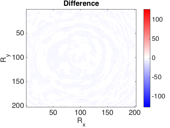
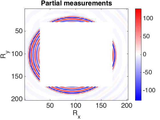
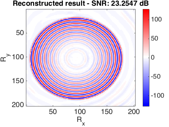
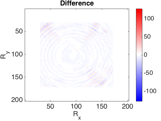
The frequency slices used in this work are generated using finite differences from the 3D Overthrust model. The data volume has \(202 \times 202\) receivers and \(102 \times 102\) sources sampled on a \(25\) m grid. We extract the \(5.31\) Hz frequency slice. For training dataset we tried to choose as little randomly selected slices as possible to achieve desired recovery accuracy. In our first experiment, we defined \(S_X\) to be the set of \(250\) slices with \(90\)% randomly missing entries (varying sampling mask) and \(250\) column-wise missing entries with the same sampling rate. In the second experiment, in order to show the capability of our method to recover from large contiguous areas of missing data (e.g. because of a platform), we recover frequency slices that miss half of their samples as a square in the middle. In this case \(S_X\) consists of \(2000\) slices. Figure 1 shows the recovery for the real part of a single slice, for these experiments. The average reconstruction SNR of slices not in the training dataset is shown in the table 1. Based on the results obtained and the number of training samples used in second experiment, we can observe that the quality of reconstruction is lower when we have large gaps in the observed data. Since other methods have not reported success in reconstructing this type of missing data, the recovery is reasonable.

Missing type	Missing percentage	Average recovery SNR (dB)
Column-wise	90%	33.7072
Randomly	90%	29.6543
Square	50%	20.6053

Discussion and conclusions

We introduced a deep learning scheme for reconstruction of heavily sub-sampled seismic data. By giving up linearity and using an adaptive nonlinear model, we are able to reconstruct seismic data with arbitrarily type of sampling that no other method is capable of. Although in order to achieve this result, we assumed that training data is available, which requires having a small percentage of shots fully-sampled. In the first experiment we showed that by recording \(5\)% of shots in random locations with a desired sampling rate, we are able to reconstruct all the other slices (in some frequency) with \(90\)% randomly or column-wise missing entries. In the next step, we are looking forward to incorporate this scheme in multiple prediction.

Acknowledgements

This research was carried out as part of the SINBAD II project with the support of the member organizations of the SINBAD Consortium.