Sparsity-promoting least-squares migration with the linearized inverse scattering imaging condition

Philipp A. Witte*, Mengmeng Yang and Felix J. Herrmann
Seismic Laboratory for Imaging and Modeling (SLIM), University of British Columbia

Introduction

Reverse-time migration (Baysal et al., 1983) has established itself as a popular technique in seismic imaging due to its capability to handle very large dips of reflectors and strong velocity contrasts. Classic reverse-time migration (RTM) uses the zero-lag cross-correlation imaging condition, which is based on the imaging principle of Clearbout (1985). In the time domain, the image is formed by cross-correlating the source and receiver wavefields, selecting the contribution at zero time shift and summing over all time steps and shots. The underlying assumption of the cross-correlation imaging condition is that the source wavefield only contains down-going events, i.e. the source is propagating in a smooth, reflection-free background model and the receiver wavefield only contains up-going events. This assumption is violated as soon as the background model contains velocity changes on a scale of the dominant wavelength, which leads to backscattering of the incident wavefield. Cross-correlating wavefields that each contain both up- and down-going events generates low-frequency contributions in the image which overlay the reflections.

Techniques for the removal of low-frequency contributions in RTM images have been an active field of research and can be classified into three main categories: filtering of the wavefields, filtering of the image and alternative imaging conditions. Filtering of wavefields is commonly done using Poynting vectors (Yoon and Marfurt, 2004) in order to separate down- and up-going events before cross-correlation (Pestana et al., 2013). In image filtering methods, such as least-squares artifact attenuation (Guitton et al., 2007) or Laplacian preconditioning (Zhang and Sun, 2009), the artifacts are removed in the image itself after cross-correlating the full source and receiver wavefields. An alternative imaging condition called linearized inverse scattering imaging condition which addresses low-frequency RTM artifacts was introduced by Op’t Root et al. (2012). This imaging condition is a partial inverse of the linearized Born scattering operator, which naturally suppresses low-frequency imaging artifacts. This method has been adopted by N. D. Whitmore and Crawley (2012) for large-scale RTM on salt models and the generation of artifact-free angle gathers (Brandsberg-Dahl et al., 2013).

The linearized inverse scattering imaging condition can be interpreted as a linear operation, which maps seismic reflection data to the image space. In this work, we first reformulate this imaging condition as the action of a linear operator and then derive its adjoint – i.e. the corresponding map from the image to the data space. This allows us to use the inverse scattering imaging condition in sparsity-promoting least-squares reverse-time migration (SPLS-RTM). LS-RTM itself tries to invert the linearized Born scattering operator, but in early iterations suffers from the low-frequency artifacts which negatively affect the convergence rate, since many of the initial iterations are spent on removing these artifacts. By using the inverse scattering imaging condition in LS-RTM, we decrease these low-frequency artifacts and improve the convergence. We address the high computational cost of LS-RTM by working with randomized subsets of sources in each iteration and we use sparsity promotion in the curvelet domain to suppress sub-sampling related artifacts.

Linearized inverse scattering imaging condition

The linearized inverse scattering imaging condition was introduced by Op’t Root et al. (2012) as a pseudo inverse as of the linearized scattering operator, which maps source and receiver wavefields to an image of the reflectors in the subsurface. Their original formulation is defined in the frequency domain and consists of a weighted sum of cross-correlated time and space derivatives of the source and receiver wavefields. Rather than formulating RTM as applying the cross-correlation imaging condition to source and receiver wavefields, we define RTM as applying the adjoint of the linearized Born scattering operator to the observed reflection data: \[ \begin{equation} \mathbf{\delta m} = \mathbf{J}^\top \mathbf{\delta d}, \label{rtm} \end{equation} \] where \(\mathbf{\delta m}\) is the model perturbation (image) and the action of the adjoint Born modeling operator on the data is defined as: \[ \begin{equation} \mathbf{J}^\top \delta \mathbf{d} = -\sum_{t} \text{diag} \Big(\ddot{\mathbf{u}}[t]\Big) \underbrace{\Big( \mathbf{A}(\mathbf{m})^{-\top} \mathcal{P}_r^\top \mathbf{\delta d} \Big) [t]}_{\mathbf{v[t]}}. \label{born} \end{equation} \] The symbol \(\mathbf{A}(\mathbf{m})\) is the discretized (acoustic) wave equation, \(\mathcal{P}_r^\top\) is the receiver data injection operator and \(\mathbf{m}\) is the background model in slowness squared. The vectors \(\mathbf{u}[t]\) and \(\mathbf{v}[t]\) are the source and receiver wavefields as a function of time and \(\ddot{\mathbf{u}}\) denotes the second time derivative of \(\mathbf{u}\). Due to readability, we omit the sum over sources in the notation.

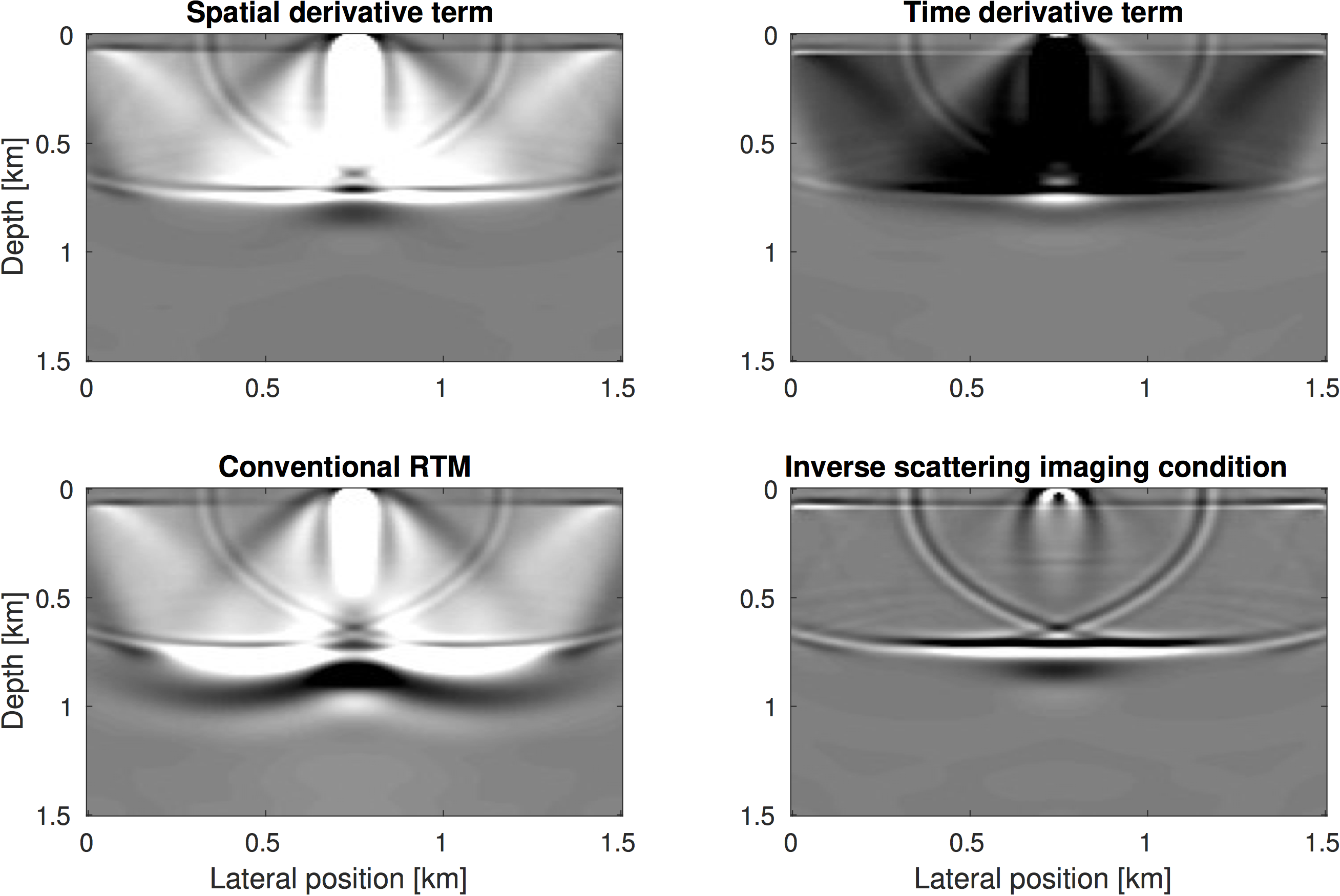
We now reformulate RTM with the inverse scattering imaging condition according to Op’t Root et al. (2012), as applying the adjoint of a new operator \(\widehat{\mathbf{J}}\) to observed reflection data: \[ \begin{equation} \widehat{\mathbf{J}}^\top \delta \mathbf{d} = \sum_{t} \Bigg\{ \text{diag} \Big(\ddot{\mathbf{u}}[t] \odot \mathbf{m} \Big) \Big( \mathbf{A}(\mathbf{m})^{-\top} \mathcal{P}_r^\top \mathbf{\delta d} \Big)[t] + \sum_{i=1}^{3} \text{diag}\Bigg( \frac{\partial \mathbf{u}[t]}{\partial \mathbf{x}_i}\Bigg) \frac{\partial}{\partial \mathbf{x}_i}\Bigg( \mathbf{A}(\mathbf{m})^{-\top} \mathcal{P}_r^\top \mathbf{\delta d} \Bigg)[t] \Bigg\}, \label{isic} \end{equation} \] where \(\frac{\partial}{\partial \mathbf{x}_i}\) is the first spatial derivative in the \(i^{\mathrm{th}}\) dimension. The first term of Equation \(\ref{isic}\) is basically equivalent to the imaging condition of the conventional adjoint Born scattering operator (Equation \(\ref{born}\)) with an additional element-wise product of \(\ddot{\mathbf{u}}\) with the model vector \(\mathbf{m}\). The second part of the inverse scattering imaging condition consists of correlating first-order spatial derivatives of the source and receiver wavefields and summing them. As discussed in N. D. Whitmore and Crawley (2012), the two terms of this expression both contain the RTM low-frequency artifacts, but with flipped signs and therefore they cancel upon summing, whereas the specular reflection events stack coherently. This is illustrated in Figure 1, where we plot the two individual terms of Equation \(\ref{isic}\), as well as their sum, for a simple two layer velocity model. The migration velocity model is a slightly smoothed version of the true model and therefore causes backscattering of the incident wavefield at the velocity interface. These artifacts pollute the RTM image, whereas they cancel out after summing the two terms of the inverse scattering imaging condition.

The benefit of writing the inverse scattering imaging condition as a linear operator is that we can easily derive the action of the forward operator, by transposing Equation \(\ref{isic}\): \[ \begin{equation} \mathbf{\delta d} = \widehat{\mathbf{J}} \delta \mathbf{m} = \Bigg\{ \mathcal{P}_r \mathbf{A}(\mathbf{m})^{-1}\text{diag} \Big( \ddot{\mathbf{u}}[t] \odot \mathbf{m} \Big)\mathbf{\delta m} + \mathcal{P}_r \sum_{i=1}^{3} \mathbf{A}(\mathbf{m})^{-1} \frac{\partial}{\partial \mathbf{x}_i} \text{diag}\Bigg( \frac{\partial \mathbf{u}[t]}{\partial \mathbf{x}_i} \Bigg)\mathbf{\delta m} \Bigg\}, \label{forward} \end{equation} \] We ensure that the implementations of \(\widehat{\mathbf{J}}\) and \(\widehat{\mathbf{J}}^\top\) are in fact a correct pair of forward and adjoint linear operators by making sure that the relation \(\langle \mathbf{y}, \widehat{\mathbf{J}} \mathbf{x}\rangle - \langle \widehat{\mathbf{J}}^\top \mathbf{y}, \mathbf{x} \rangle < \epsilon\) holds within machine precision for arbitrary vectors \(\mathbf{x}\) and \(\mathbf{y}\). These operators can then be used in iterative solvers for LS-RTM, such as LSQR or linearized Bregman.

Data example

We demonstrate the benefits of sparsity-promoting LS-RTM with the inverse scattering imaging condition in comparison to SPLS-RTM with the conventional zero-lag cross-correlation imaging condition on the Sigsbee 2A model. We choose this model because it has a large and very shallow salt body, which causes significant backscattering of energy in both source and receiver wavefields. We use the full Sigsbee model (24.3 x 9.1 km) and generate 972 shot records with 25 m shot spacing, 8 seconds recording time and 15 Hz peak frequency. Each experiment is recorded by 972 receivers that are spread out over the full model, but for imaging we limit the maximum offset to ~10 km.

Because LS-RTM with the full number of shots is very expensive, we use randomized subsets of 100 sources per iteration and sparsity promoting of the image in the curvelet domain to address subsampling artifacts. We formulate our objective using a strictly convex elastic net, which is a linear combination of \(\ell_1\) and \(\ell_2\) norms: \[ \begin{equation} \begin{aligned} &\underset{\mathbf{\delta m}}{\operatorname{minimize}} \hspace{.3cm} \lambda||\mathbf{C} \mathbf{\delta m}||_1 + \frac{1}{2} ||\mathbf{C} \mathbf{\delta m}||_2^2\\ &\text{subject to: } ||\hspace{.1cm} \widehat{\mathbf{J}} \delta \mathbf{m} - \delta \mathbf{d}||_2 \leq \sigma. \end{aligned} \label{objective} \end{equation} \] In this expression the matrix \(\mathbf{C}\) is the forward curvelet transform, \(\sigma\) is the size of the noise of the seismic data and \(\lambda\) is a weighting parameter controlling emphasis. Adding the \(\ell_2\) norm in the objective makes the function strongly convex and allows us to solve this problem with the linearized Bregman method (Yin, 2010), which offers flexibility to work with different randomized subsets for each iteration. For details on seismic imaging with the linearized Bregman method refer to Herrmann et al. (2015).

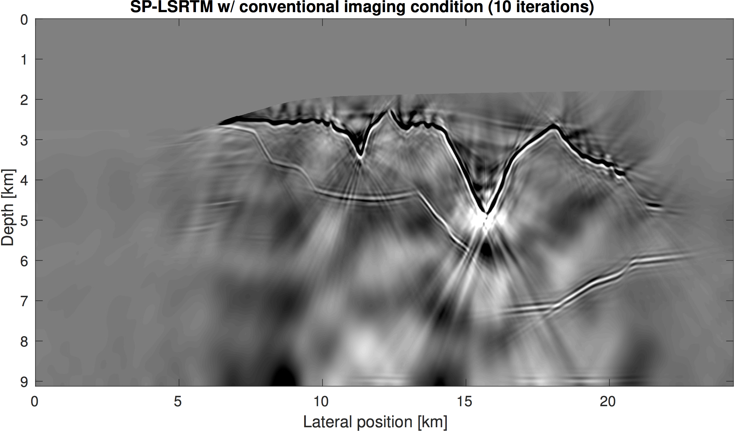
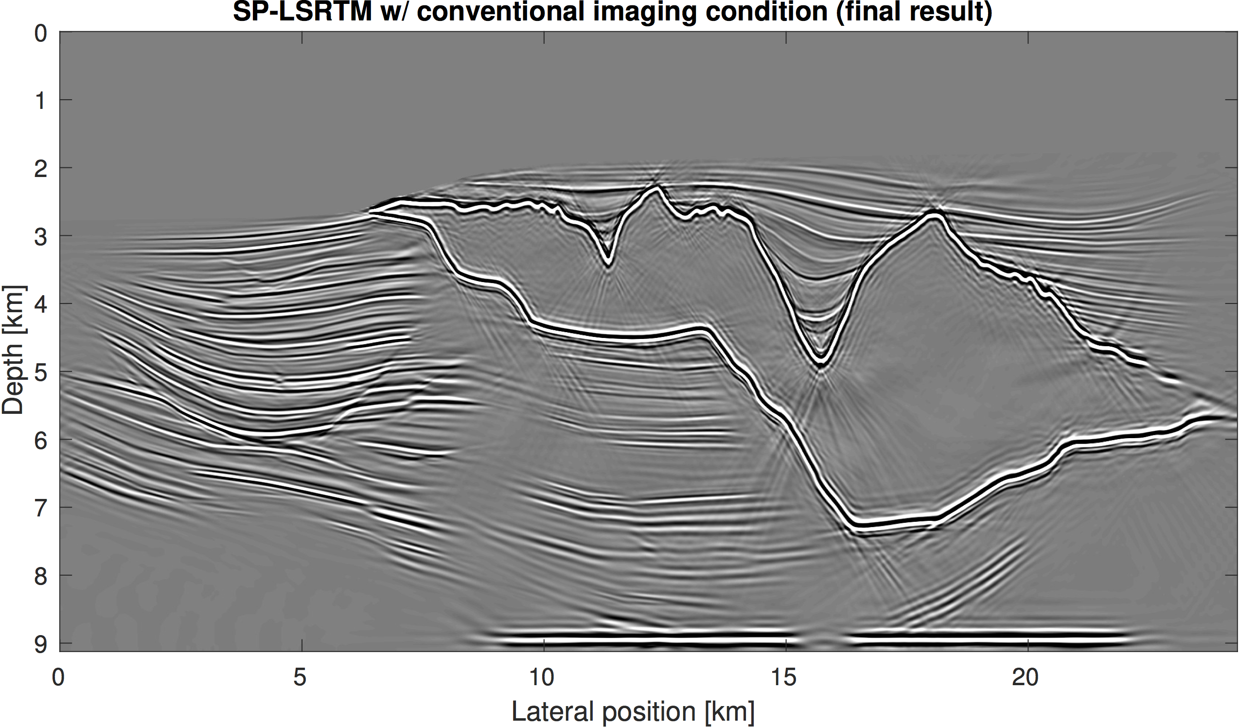
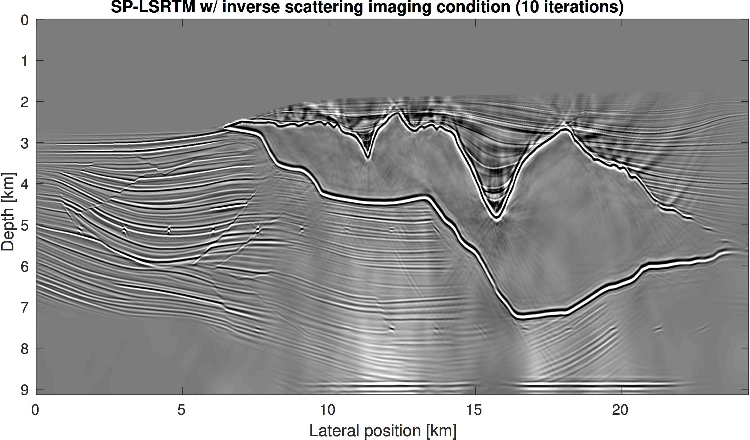
The linearized Bregman method only requires matvec actions of \(\widehat{\mathbf{J}}\) and \(\widehat{\mathbf{J}}^\top\), which we have defined in the previous section. In our experiment, we compare SPLS-RTM using the conventional linearized Born scattering operator \(\mathbf{J}\) and our modified operator \(\widehat{\mathbf{J}}\). The observed reflection data sets for the two cases are each generated with their corresponding operator (inverse crime). We furthermore use some basic preconditioners, namely a model space linear depth scaling, muting of long offsets and the ocean bottom reflection and muting of the water column in the image space. However, we do not use Laplacian preconditioning or any other type of filter on the image during inversion. Intermediate results for both experiments after 10 iterations are plotted in the left hand column of Figure 2. SPLS-RTM with the inverse scattering imaging condition was able to remove the low-frequency artifacts significantly better than conventional SPLS-RTM. Since the result of conventional SPLS-RTM after 10 iterations is so poor, we run a total of 25 iterations, but we run no further iterations of sparsity-promoting LS-RTM with the inverse scattering imaging condition. For the comparison of the final results (right hand column of Figure 2) we apply a post-migration Laplace filter to both images to remove any residual artifacts. The SPLS-RTM image using the inverse scattering imaging condition has higher resolution, contains more sub-salt reflectors and resolves the point-diffractors, which are completely absent in the image of SPLS-RTM with the cross-correlation imaging condition.

Using the inverse scattering imaging and modeling operators does not require additional memory in comparison to the conventional Born scattering operator, as the spatial derivative terms are computed on the fly. Therefore this method can be applied to large-scale 3D imaging problems.

Conclusions

We have reformulated the linearized inverse scattering imaging condition as the action of an adjoint linear operator that acts on observed data. This imaging condition is a pseudo inverse of the linearized scattering operator and naturally suppresses low-frequency artifacts that appear in RTM images and LS-RTM gradients. We derive the corresponding forward operator of this imaging operator, which allows us to incorporate the inverse scattering imaging condition into sparsity-promoting LS-RTM. We demonstrate on the Sigsbee 2A model, that low-frequency imaging artifacts are significantly reduced in comparison to SPLS-RTM with the cross-correlation imaging condition and sub-salt point-diffractos are resolved in the image. The method is furthermore not more intensive than conventional LS-RTM and together with our sparsity promoting LS-RTM algorithm with source subsampling, can be applied to large-scale 3D problems. As future research, we plan to include a curvelet-domain matched filtering procedure, such that the cancelation of low-frequency artifacts in these terms is further improved.

Acknowledgements

This research was carried out as part of the SINBAD II project with the support of the member organizations of the SINBAD Consortium. The authors wish to acknowledge the SENAI CIMATEC Supercomputing Center for Industrial Innovation, with support from BG Brasil, Shell, and the Brazilian Authority for Oil, Gas and Biofuels (ANP), for the provision and operation of computational facilities and the commitment to invest in Research & Development.