Improved time-lapse data repeatability with randomized sampling and distributed compressive sensing

Introduction

Time-lapse (4D) seismic technology has been used extensively for monitoring a variety of subsurface changes including fluid flow in producing reservoirs (D. E. Lumley, 2001). A crucial part of 4D processing involves achieving prestack time-lapse data repeatability, which is also important for AVO purposes (Houck, 2007; Harris and Veritas, 2005). Repeatability is dependent on several factors including the similarity in the time-lapse survey geometries and subsequent processing workflow. To this end, considerable effort is spent on ensuring significant replicability amongst the time-lapse (baseline and monitor) surveys (Eiken et al., 2003), in order to achieve acceptable levels of repeatability expressed in normalized RMS (NRMS)(Kragh and Christie, 2002). However, the practice of replicating time-lapse surveys that yield vintages with excellent repeatability remains challenging because of unavoidable differences in acquisition such as differences in noise between surveys (Ross et al., 1997; Rickett and Lumley, 2001). Using ideas from compressive sensing (CS), several authors (F. J. Herrmann, 2010; Hennenfent and Herrmann, 2008; Mansour et al., 2012) show that randomized sampling can reduce the cost of seismic data acquisition with increase in the fold. This observation is supported by Mosher et al. (2014) who demonstrated similar approach in the field showing its implications for acquisition cost reduction compared to conventional methods for seismic data acquisition—up to ten-fold improvements in economics and environment impact with improvements in resolution.

Following remarkable success with CS-based acquisition technology, Oghenekohwo et al. (2014) proposed randomized sampling for time-lapse acquisition and a joint recovery model (JRM) to address challenges related to cost of the surveys and difficulty in replicating surveys. The JRM which derives from distributed compressive sensing (DCS) (Baron et al., 2009), recovers a common part and innovations with respect to the common part, leading to improved recovery of time-lapse vintages when the surveys are not replicated. The authors confirmed this observation using an example of a CS-based acquisition design—time-jittered sources in marine (Wason and Herrmann, 2013). However, accurate recovery of seismic data in CS hinges on precise knowledge of the acquisition parameters including the relative precise information on source/receiver coordinates. When two independent samplings are acquired over an earth that did not change—no time-lapse—the recovery from the vintages should not show differences in the difference panel and exhibit high levels of repeatability or low NRMS values. Therefore, we leverage NRMS as a reliable QC to measure repeatability of vintages from non-replicated acquisitions that are recovered using JRM under two distinct cases. First, we show recovery and compute the repeatability of vintages from measurements corrupted with swell noise in situations where we have precise information of the source/receiver locations. Next we conduct experiments without noise but where there are moderate calibration errors i.e., errors that arise where our recorded source/receiver coordinates do not match the exact coordinates measured in the field. We present results on a seismic receiver gather in a fixed-spread acquisition configuration with time-jittered sources in a marine setting.

Compressed sensing time-lapse acquisition

Time-lapse seismic acquisition with two independent surveys, denoted by \(j=1\) (baseline) and \(j=2\) (monitor), can be modeled as: \(\vd{y}_{j} = \vd{A}_{j}\vd{x}_{j}\ \text{for}\ j=\{1,2\},\) where \(\vd{y}\) is the observed undersampled and “compressed” data. In general , we define \(\vd{A}_{j} = \vd{R}_{j}\vd{M}\tensor{C}^H\) following existing work by (F. J. Herrmann, 2010; Hennenfent et al., 2010; Mansour et al., 2012); where \(\vd{M}\) is a measurement matrix; \(\vd{R}\) is a restriction operator that is different for the time-lapse acquisitions; \(\vd{x}\) is a sparse/compressed representation of the densely sampled data \(\vd{d}\); hence, \(\vd{d} = \tensor{C}^H \vd{x}\), with \(\tensor{C}\) being the curvelet transform and the superscript \(H\) denotes the conjugate transpose. When the observed data is noisy, the equation becomes: \(\vd{y}_{j} = \vd{A}_{j} \vd{x}_{j} + \vd{n}_{j}\), where \(\vd{n}\) is the noise and is different for either acquisition. In CS-based seismic data recovery, our goal is to recover an approximation of \(\vd{x}\). In the noise-free case, we achieve this objective by solving the sparsity-promoting program: \(\widetilde{\vd{x}} = \argmin_{\vd{x}}\|\vd{x}\|_1 \quad \text{subject to} \quad \vd{y} = \vd{Ax}, \) for \(j\in {1,2}\). Rather than follow an independent recovery strategy (IRS), where we recover \(\widetilde{\vd{x}}_1\) and \(\widetilde{\vd{x}}_2\) separately, we adopt the joint recovery model (JRM) proposed by Oghenekohwo et al. (2014) for processing time-lapse data using shared information among the vintages. This model derives from distributed compressed sensing (DCS) (Baron et al., 2009) and instead involves the following system of equations: \[ \begin{equation} \begin{aligned} \begin{bmatrix} \vd{y}_1\\ \vd{y}_2\end{bmatrix} &= \begin{bmatrix} {\vd{A}_1} & \vd{A}_{1} & \vd{0} \\ {\vd{A}_{2} }& \vd{0} & \vd{A}_{2} \end{bmatrix} \begin{bmatrix} \vd{z}_0 \\ \vd{z}_1 \\ \vd{z}_2 \end{bmatrix},\quad\text{or} \quad \vd{y} = \vd{A}\vd{z}\\ \end{aligned} \label{jrmobs} \end{equation} \] by minimizing \(\widetilde{\vd{z}} = \argmin_{\vd{z}}\|\vd{z}\|_1\DE\sum_{i=1}^N|z_i| \quad \text{subject to} \quad \vd{y} = \vd{Az}. \) In this expression, the vector \(\vd{z}_0\) contains the common component and \(\vd{z}_j\) for \(j\in {1,2}\) are the innovations with respect to the common component that is shared by the vintages. Subsequently, estimates of \(\widetilde{\vd{x}}_1\) and \(\widetilde{\vd{x}}_2\) are computed from recovery of these three components. Under certain assumptions, Oghenekohwo et al. (2014) and Wason et al. (2015) showed that (i) independent non-replicated time-lapse surveys (\(\vd{A}_1 \neq \vd{A}_2\)) yield better recoveries for the vintages when processed jointly with the JRM and the results are superior to those obtained with the IRS and (ii) when the surveys are calibrated, we get results that are more or less equivalent to results when repeating the surveys exactly. This is case for time lapse while vintages improve.

Time-lapse repeatability

A common practice in time-lapse seismic processing involves measuring the repeatability of the observed and processed data at every subsequent processing step (Ross et al., 1997; Houck, 2007; Harris and Veritas, 2005). Repeatability measures the similarity between two traces, say \(\vd{x}_1\) from the baseline, and \(\vd{x}_2\) from the monitor. It can be measured using the normalized RMS (Kragh and Christie, 2002) defined as the ratio of the RMS of the difference of two traces to the mean of the RMS of the traces—i.e., \(\text{NRMS} (\vd{x}_1,\vd{x}_2) = \dfrac{ 2 \times \text{RMS}(\vd{x}_1-\vd{x}_2)}{\text{RMS}(\vd{x}_1)+\text{RMS}(\vd{x}_2)}.\) As a result, NRMS values ranges between 0 and 200 when expressed as a percentage. The smaller the percentage (lower NRMS), the more repeatable the traces are. In general, NRMS values are computed using traces extracted from the data in a common time window and frequency band where there are no time-lapse changes. We leverage the latter requirement in our experiments to quantify the repeatability of the recovered data in the situation where the earth does not change but where the noise and randomized independent acquisitions differ (\(\vd{A}_1 \neq \vd{A}_2\)). We compare results using the IRS to those from JRM in order to further validate the performance of the JRM.

Experiments

We consider a fixed spread seismic data acquisition with ocean bottom receivers, using time-jittered sources—a CS inspired acquisition design. Here, a receiver gather, for instance, shows overlapping shots that are unraveled and interpolated during the seismic data recovery stage (Wason and Herrmann, 2013). In the noise-free case and without calibration, Oghenekohwo et al. (2014) and Wason et al. (2015) showed that independent and non-replicated acquisitions lead to improved recovery of the time-lapse vintages using the JRM over IRS. Their observations motivate us to investigate the role of calibration errors and noise within CS-based time-lapse acquisition design. We achieve this by conducting two classes of experiments on an earth model that does not change and compute the repeatability in terms of NRMS. Because there is no time-lapse change, any errors in the recovered data may be attributed to acquisition differences and/or recovery method. In all the experiments, the acquisitions are not replicated (\(\vd{A}_1 \neq \vd{A}_2\)), meaning we do not repeat the same jittered source locations in the two time-lapse surveys.

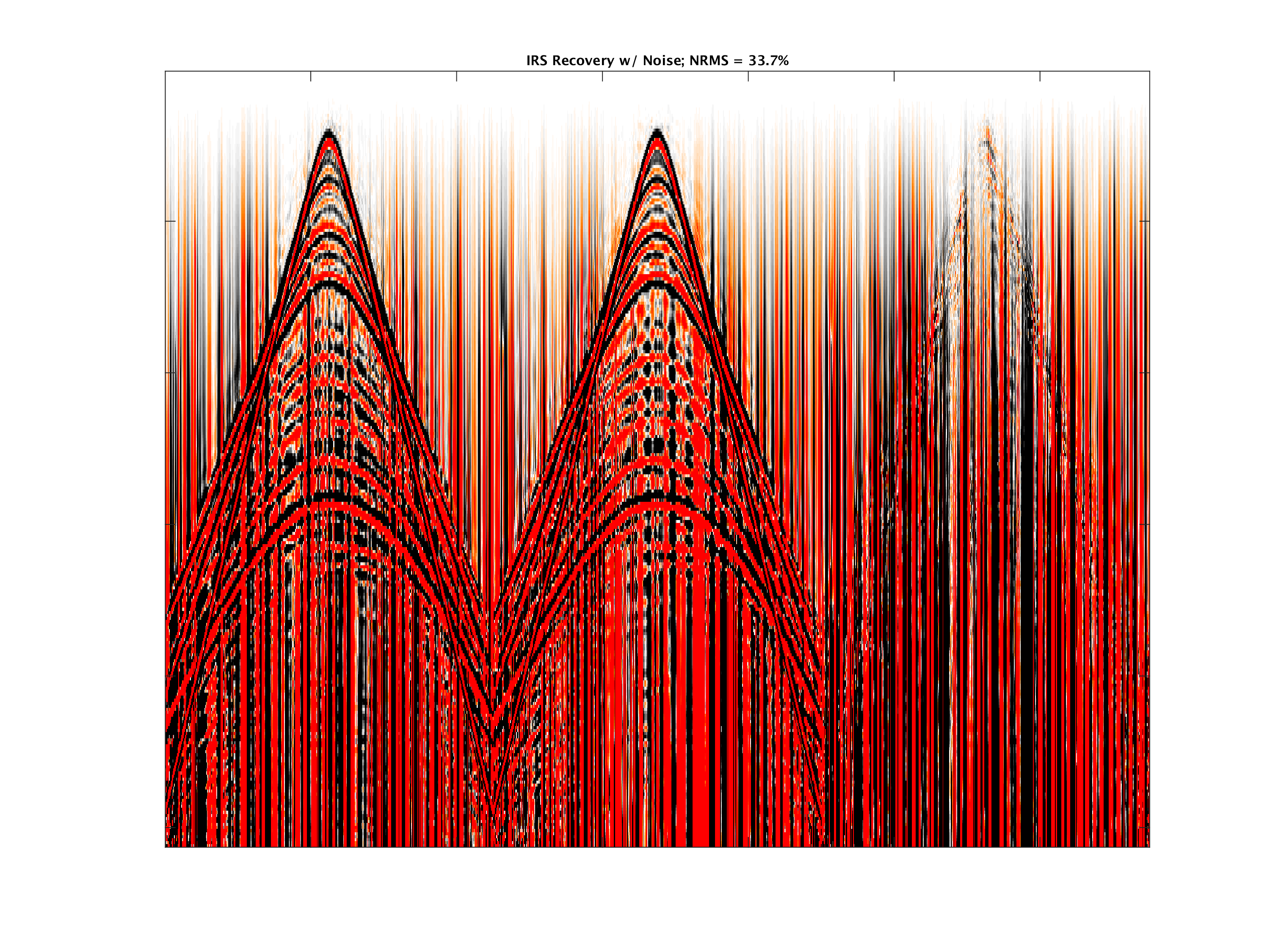
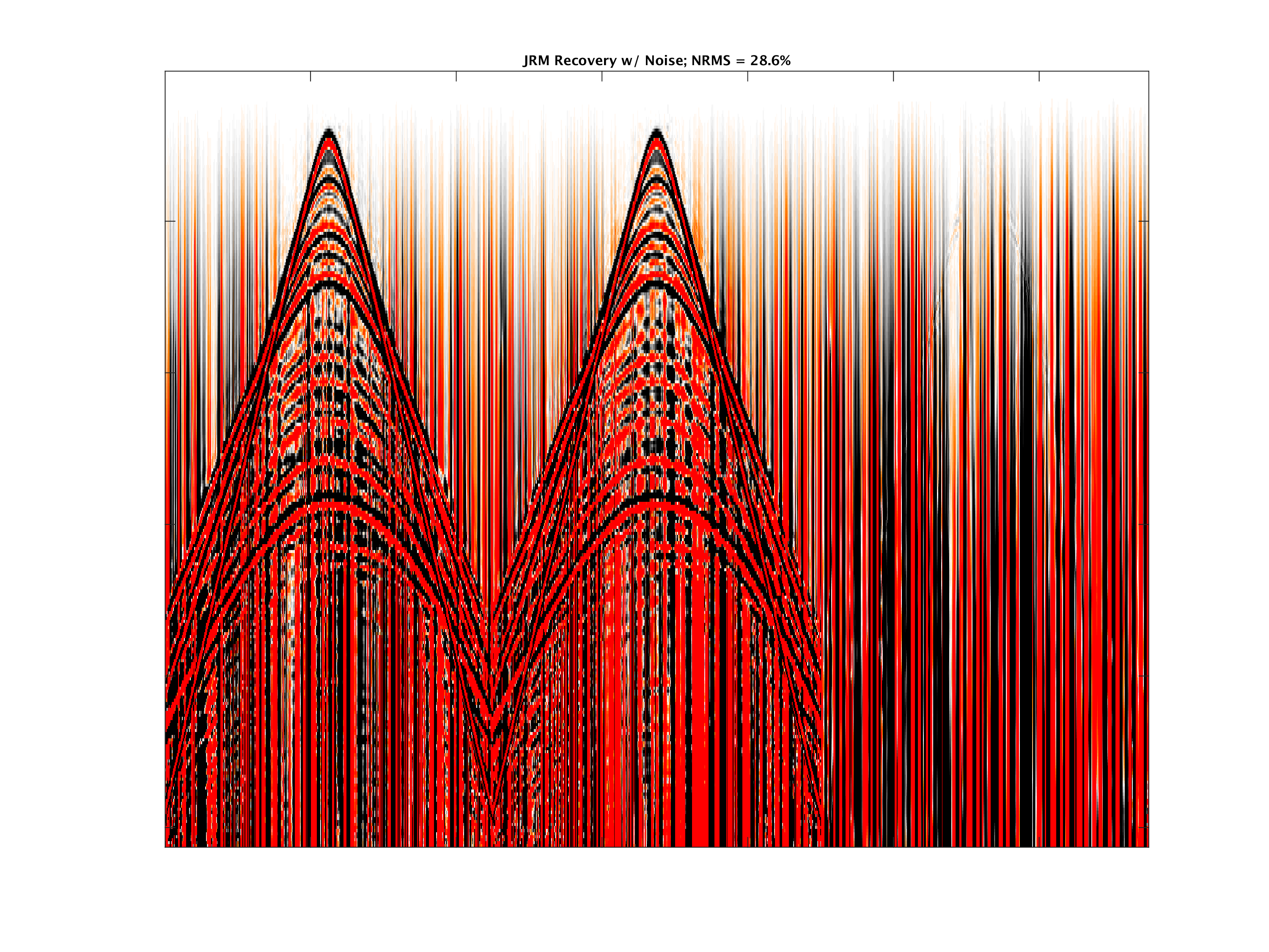
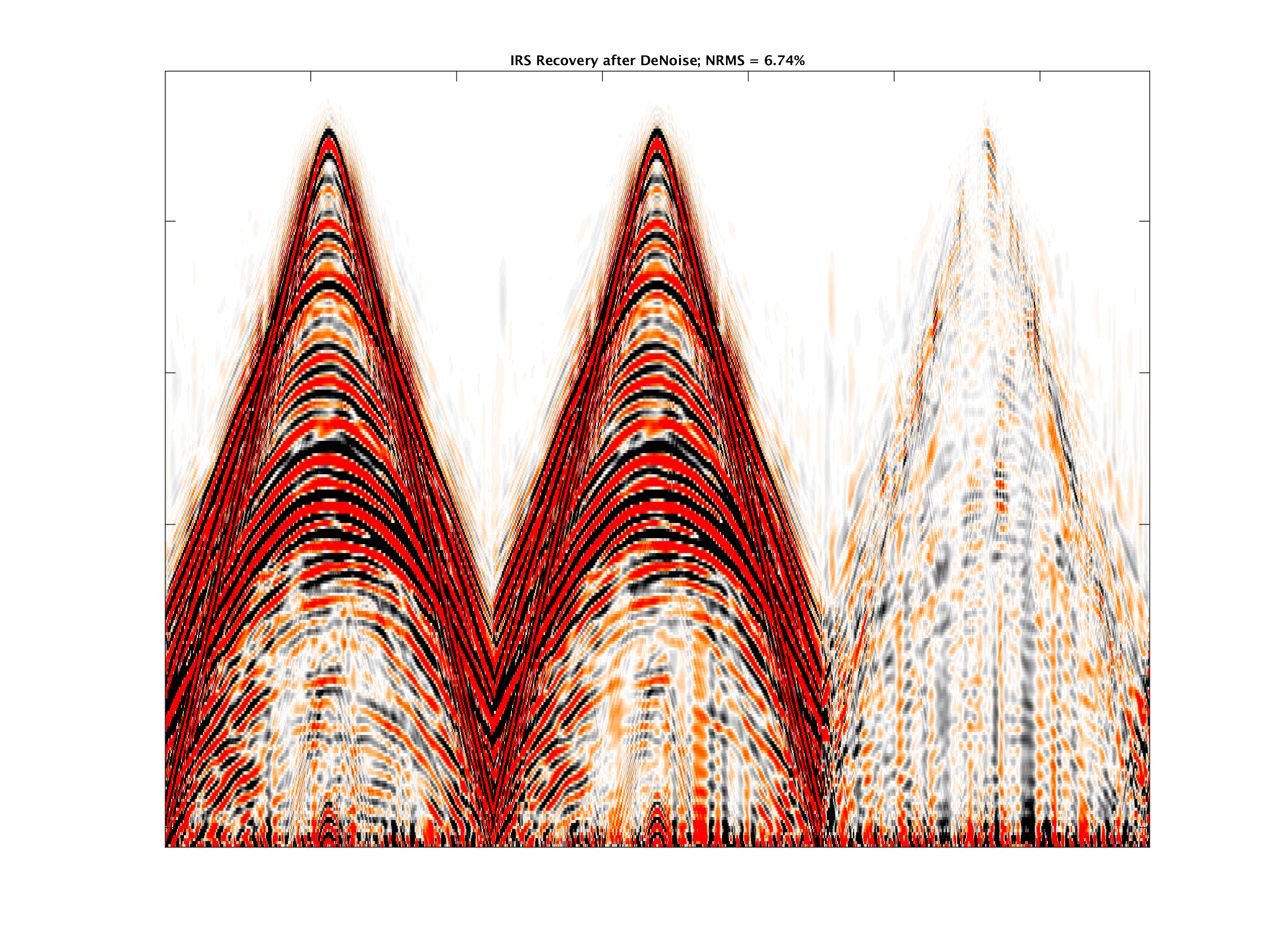
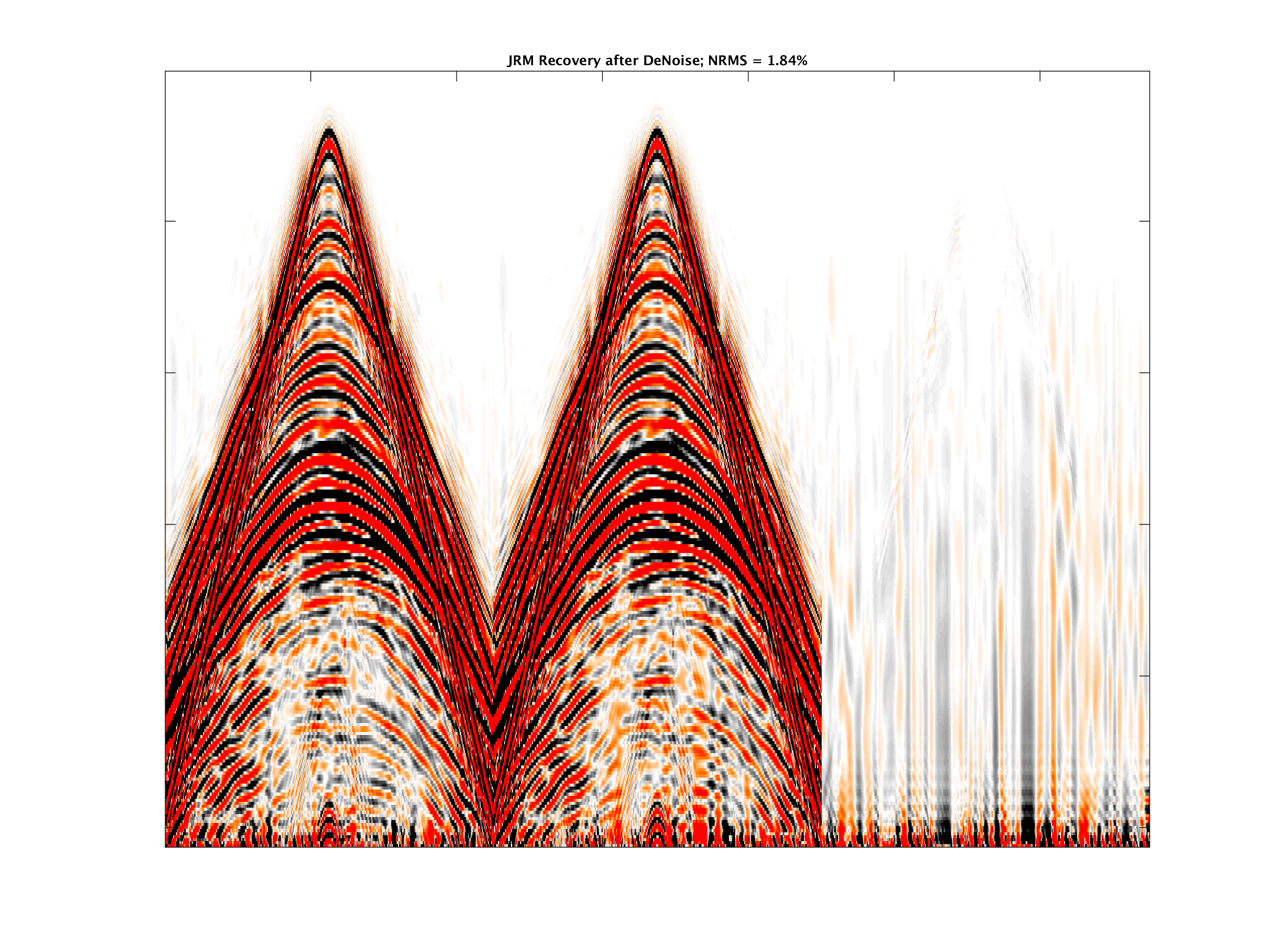
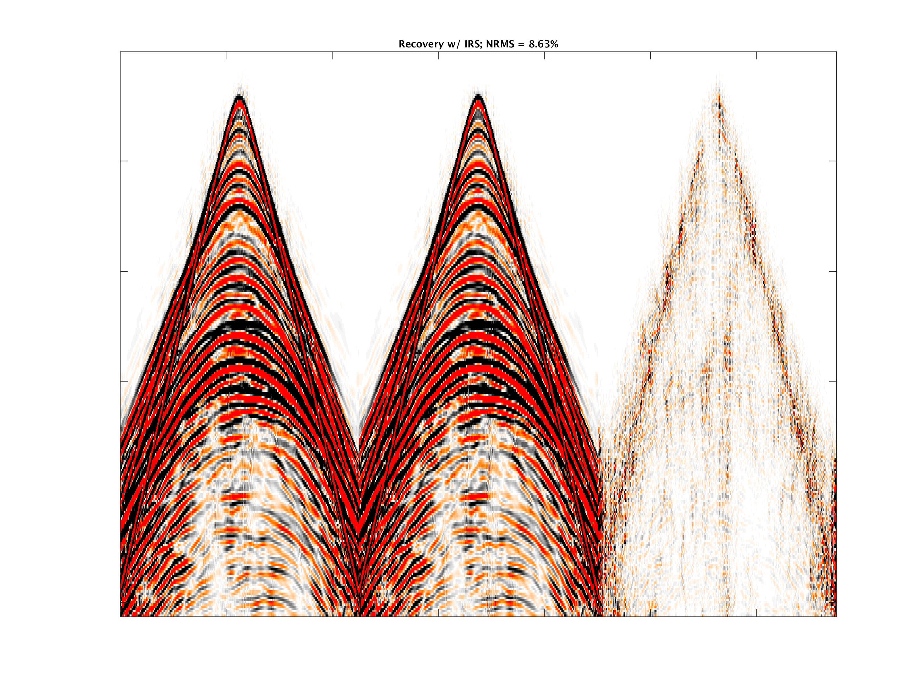
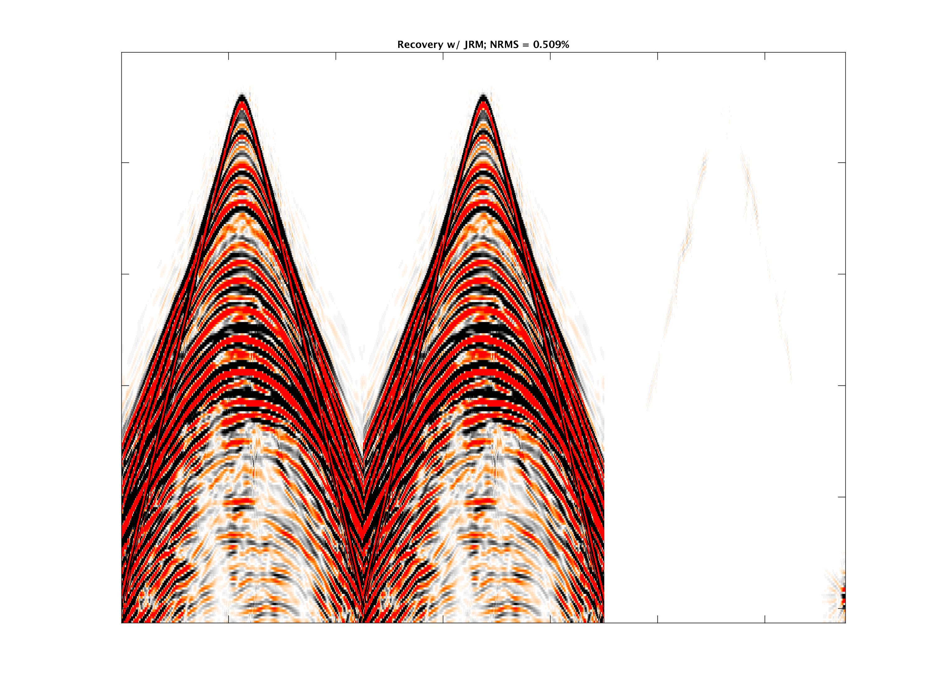
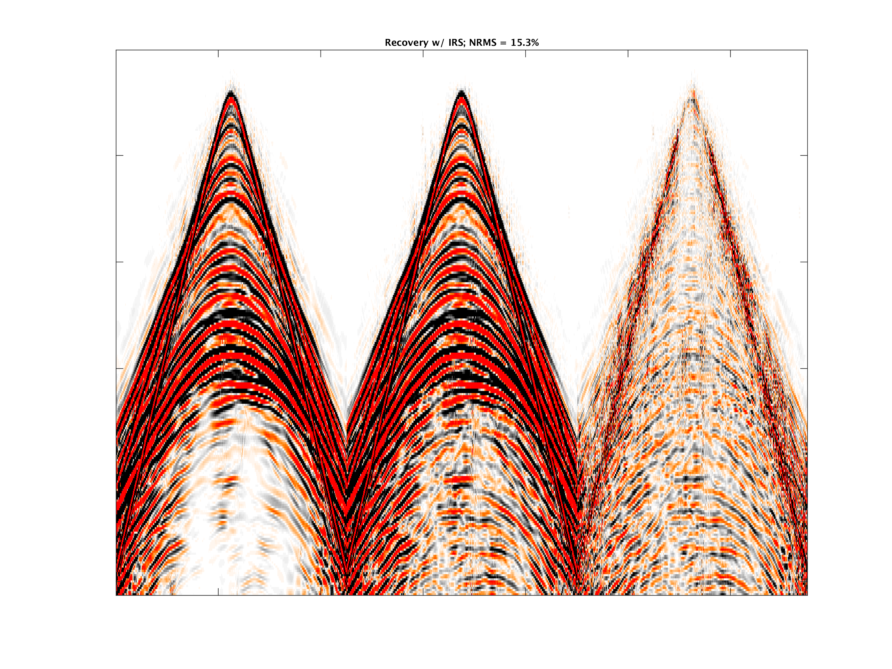
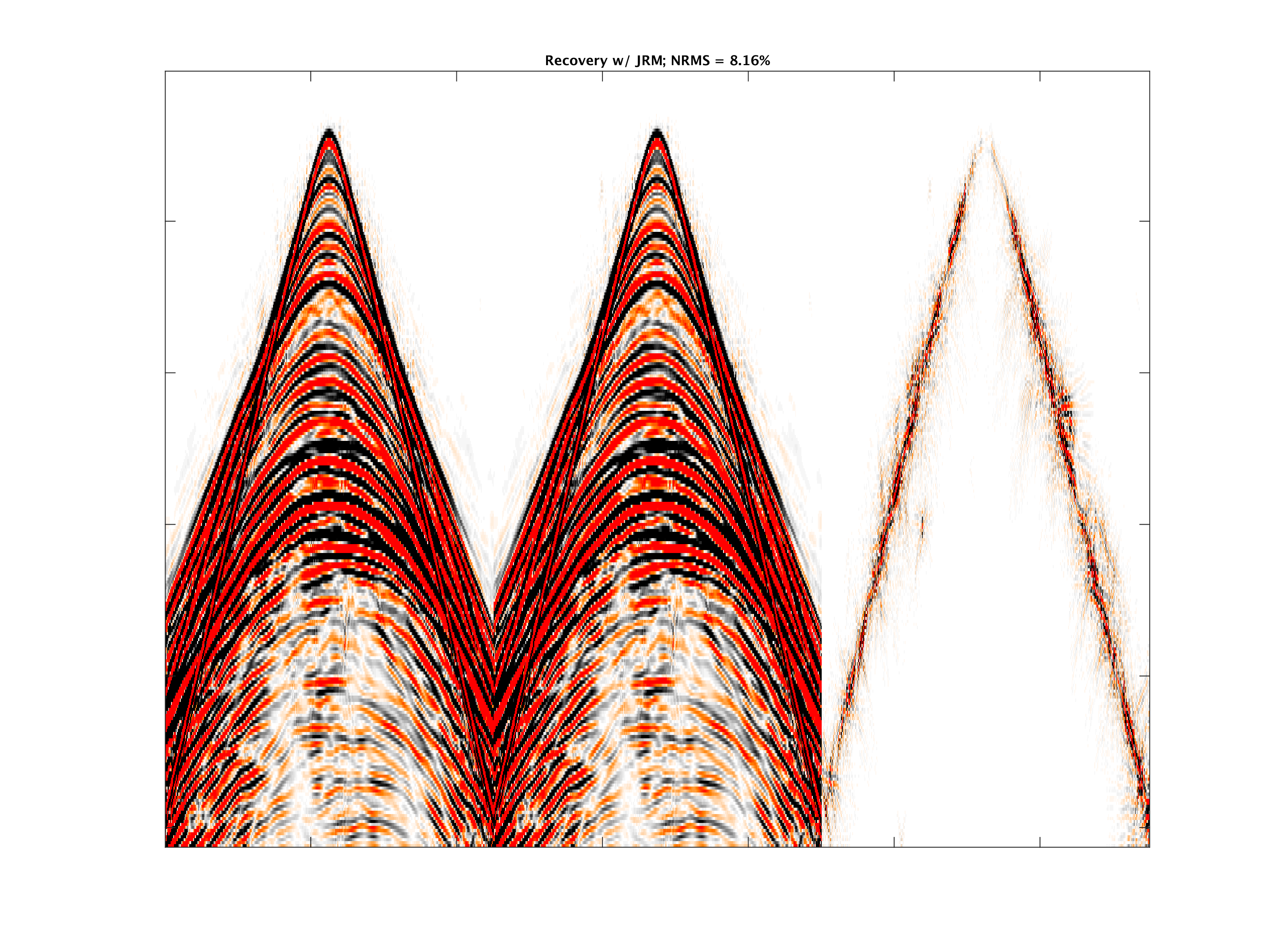
Two different sets of “compressed” subsampled seismic data (on a receiver gather) are acquired from the same earth model with geometries corresponding to different jittered source locations. Next, a different set is generated by adding different realizations of swell noise to the first set of data. We first conduct experiments on the latter, without any calibration error, so that the only observable difference after recovery is the difference in noise as shown in the top row of Figure 1. In all the plots, the third panel is the difference between first two panels after recovery with IRS or JRM. Although no coherent energy is lost, the noise is still present accounting for the high values of NRMS. However, a simple \(f-k\) filtering of the noise improves the repeatability significantly afterwards, with the JRM showing the best NRMS values. In the second experiment, we address the issue of calibration. Recall this corresponds to the situation where we have no precise knowledge of the acquisition information leading to moderate errors in both \(\vd{A}_1\) and \(\vd{A}_2\). In this example, we allow for errors up to \(2.5m\) between the recorded and exact source locations, in both acquisitions. At the top of Figure 2, we present results with IRS and JRM when there are no calibration errors—the recorded and true coordinates coincide—showing excellent repeatability with the JRM. This result is not surprising since recovery with CS relies on precise knowledge of the geometry. On the other hand, when we allow calibration errors, the repeatability with IRS degrades significantly while that of JRM does not.

Conclusion

We have shown that higher levels of repeatability are attainable from independent time-lapse surveys with randomized sampling. In situations where the earth does not change but noise and acquisition differ between surveys, using the NRMS as a QC for measuring repeatability, we show that our joint recovery model can address issues related to noise in CS-based time-lapse surveys. We confirm this by computing the NRMS of the recovered vintages using our model and compare the results to an independent processing approach that performs poorly. We also show that our approach can handle calibration errors that arise from mismatch between actual and recorded source/receiver coordinates. Finally, our findings is a prediction that CS-based time-lapse acquisition is feasible.

Acknowledgements

This research was carried out as part of the SINBAD II project with the support of the member organizations of the SINBAD Consortium.