Compressed sensing in 4-D marine—recovery of dense time-lapse data from subsampled data without repetition

Introduction

Simultaneous (or blended) marine acquisition is being recognized as an economic way to sample seismic data and speedup acquisition, wherein single and/or multiple source vessels fire shots at random times resulting in overlapping shot records (Kok and Gillespie, 2002; Beasley, 2008; Berkhout, 2008; Hampson et al., 2008; Moldoveanu and Quigley, 2011; Abma et al., 2013). Deblending (or source separation) then aims to recover unblended data, as acquired during conventional acquisition, from blended data. Wason and Herrmann (2013) showed that compressed sensing (CS) is a viable technology to sample seismic data economically and proposed an alternate sampling strategy for simultaneous acquisition (time-jittered marine), addressing the deblending problem through a combination of tailored (blended) acquisition design and sparsity-promoting recovery via convex optimization using \(\ell_1\) constraints. Here, deblending interpolates the sub-Nyquist, jittered shot positions to a fine regular grid while unraveling the overlapping shots. The implications of randomization in time-lapse (or 4-D) seismic, however, are less well-understood since the current paradigm relies on dense sampling and repeatability amongst the baseline and monitor surveys (Lumley and Behrens, 1998). These requirements impose major challenges because the insistence on dense sampling may be prohibitively expensive and variations in acquisition geometries (between the surveys) due to physical constraints do not allow for exact repetition of the surveys.

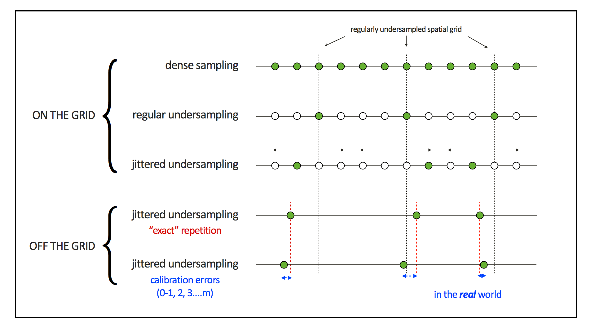
In this paper, we extend our work on time-jittered marine acquisition to time-lapse surveys for more realistic field acquisitions on irregular spatial grids, where the notion of exact repetition between the surveys is inexistent. This is because the “real” world suffers from “calibration errors”—i.e., errors due to the difference between pre- and post-acquisition shot (and/or receiver) locations on irregular spatial grids, rendering exact repetition (or overlap) between the surveys impossible. Also, since we are always subsampled in both the baseline and monitor surveys, we are interested in recovering the densely sampled vintages and the 4-D difference from subsampled/incomplete baseline and monitor data. To accomplish this, we use recent insights from distributed compressed sensing (DCS, Baron et al. (2009)), wherein the joint recovery framework exploits the fact that the signals to be recovered share a lot of information, which is typical of the data acquired during the baseline and monitor surveys. The presented scenario is different from the current paradigm where a dense baseline and a subsampled monitor are acquired, and the 4-D difference is then computed by the difference of traces shared by the dense baseline and the subsampled monitor. In our case, we work with subsampled baseline and monitor data on irregular grids, without insisting on repeatability and while knowing where the samples were taken, to recover the dense vintages first (on a fine regular grid) and then recover the complete 4-D difference.

Compressed sensing

Compressed sensing (CS, Donoho, 2006) is a novel nonlinear sampling paradigm in which randomized sub-Nyquist sampling (assuming periodic underlying grid) is used to capture the structure of the data/signal that have a sparse or compressible representation in some transform domain—i.e., if only a small number k of the transform coefficients are nonzero or if the data can be well approximated by the k largest-in-magnitude transform coefficients. For a high-dimensional signal \(\vector{f}_0 \in \mathbb{R}^N\), which admits a sparse representation \(\vector{x}_0\) in some transform domain \(\vector{S}\) (then \(\vector{f}_0 = \vector{S}^\vector{H} \vector{x}_0\), where \(^\vector{H}\) denotes the Hermitian transpose), the goal in CS is to obtain \(\vector{f}_0\) (or an approximation) from nonadaptive linear measurements \(\vector{y} = \vector{Af}_0\), where \(\vector{A}\) is an \(n \times N\) measurement matrix with \(n \ll N\). Utilizing prior knowledge that \(\vector{f}_0\) is sparse—i.e., \(\vector{x}_0\) is sparse, CS aims to find an estimate \(\tilde{\vector{x}}\) (for the underdetermined system of linear equations: \(\vector{y} = \vector{Af}_0\)) by solving the basis pursuit (BP) convex optimization problem: \[ \begin{equation} \label{eqBP} \tilde{\vector{x}} = \argmin\limits_{\vector{x}} \|\vector{x}\|_1 \quad \text{subject to} \quad \vector{y} = \vector{Ax}, \end{equation} \] where the \(\ell_1\) norm \(\|\vector{x}\|_1\) is the sum of absolute values of the elements of a vector \(\vector{x}\). With the inclusion of the sparsifying transform, the matrix \(\vector{A}\) can be factored into the product of an \(n \times N\) sampling (or acquisition) matrix \(\vector{M}\) and the synthesis matrix \(\vector{S}^\vector{H}\)—i.e., \(\vector{A} = \vector{MS}^\vector{H}\). Note that this assumes a periodic underlying grid, whereas in-field acquisitions lie on irregular grids due to calibration errors and maybe due to the acquisition design itself.

Time-lapse marine acquisition via jittered sources

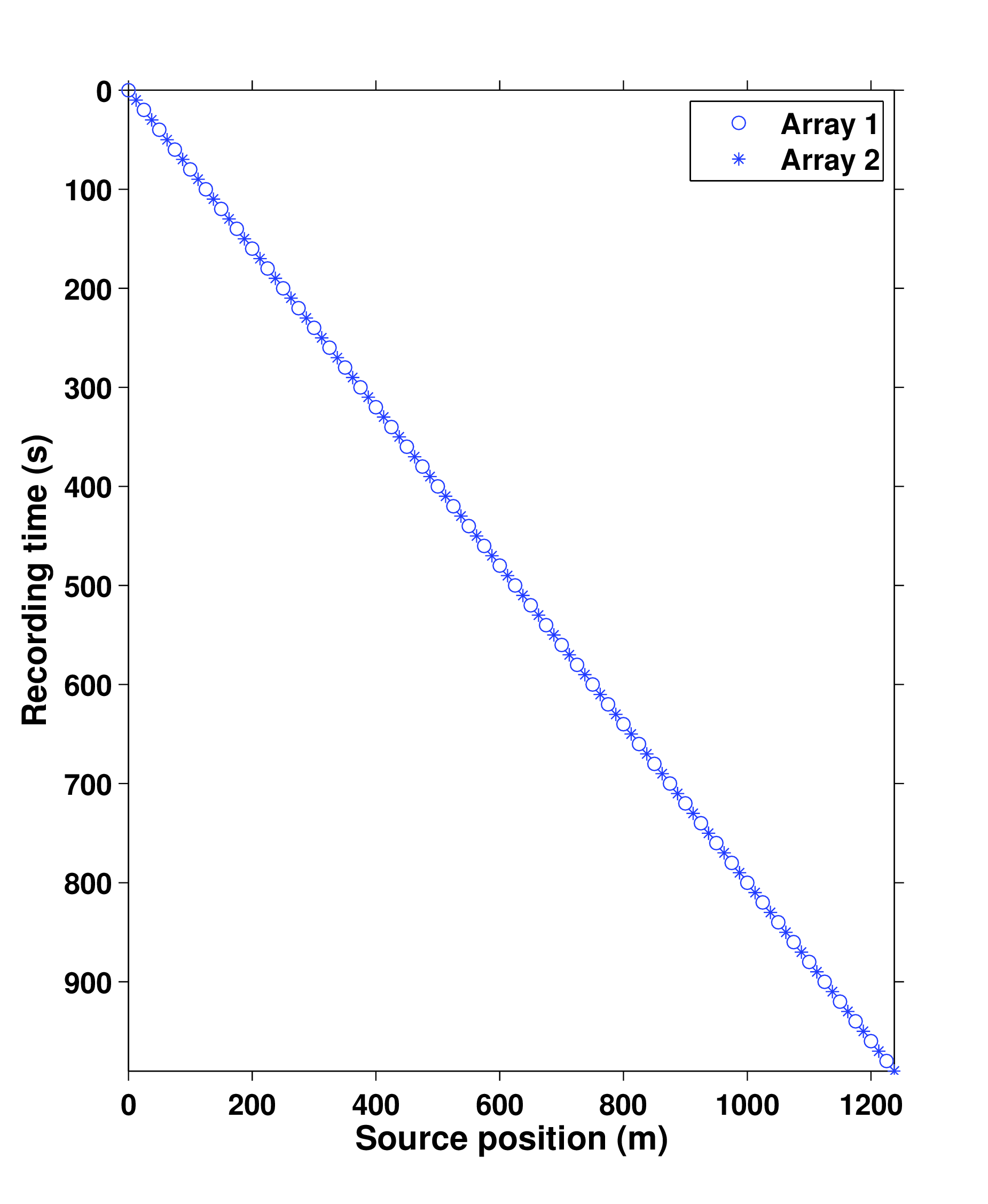
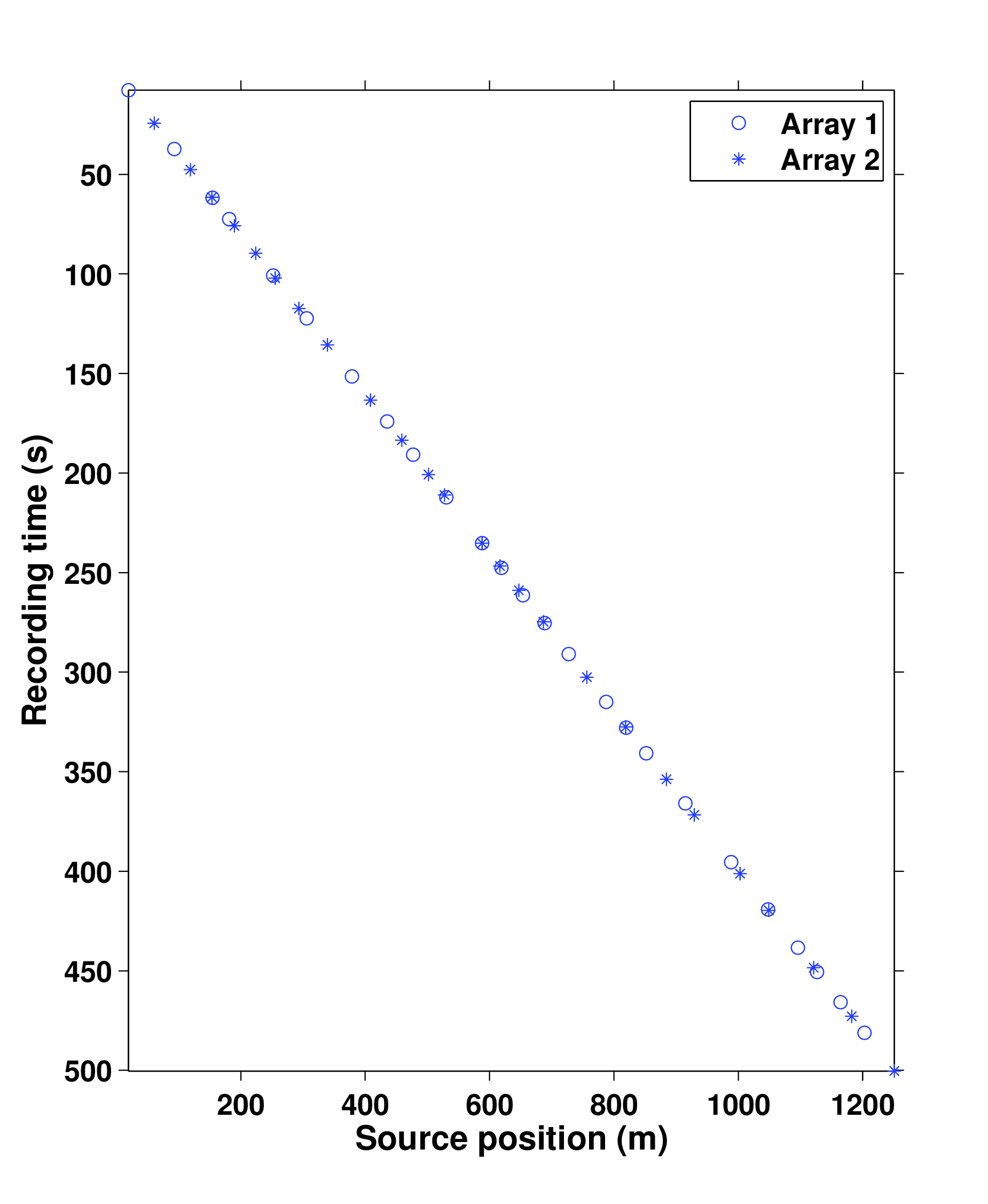
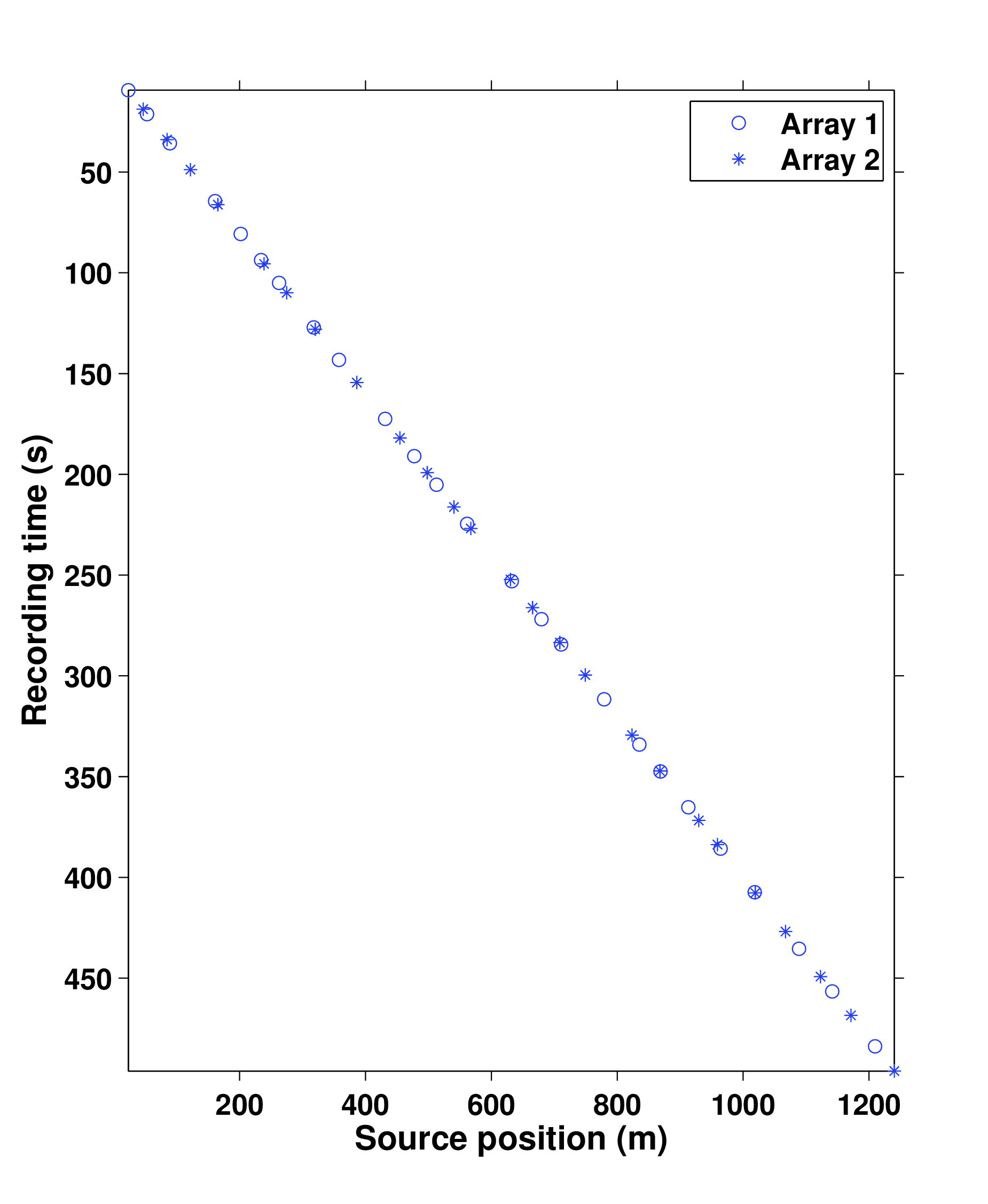
Wason and Herrmann (2013) presented a pragmatic simultaneous marine acquisition scheme, termed as time-jittered marine, that leverages CS by invoking randomness in the acquisition via random time jittering. In this acquisition a single (or multiple) source vessel maps the survey area firing shots at jittered time-instances, which translate to jittered shot locations for a given speed of the source vessel. The receivers (OBC/OBN) record continuously resulting in blended shot records. Detailed explanation of the acquisition design can be found in their paper. Figure 1 illustrates the different subsampling schemes on and off the grid. Figure 2a illustrates a conventional marine acquisition scheme and two realizations of the off-the-grid time-jittered marine acquisition are shown in Figures 2b and 2c, one each for the baseline and the monitor survey. Note that these are incomplete/subsampled acquisitions, and exact repetition of the surveys is not possible due to calibration errors.

We describe noise-free time-lapse data acquired from a baseline and a monitor survey as \(\vector{y}_{j} = \vector{A}_{j}\vector{x}_{j}\) for \(j=\{1,2\}\), where \(\vector{y}_1\) and \(\vector{y}_2\) represent the subsampled, blended measurements for the baseline and monitor surveys, respectively; \(\vector{A}_1\) and \(\vector{A}_2\) are the corresponding flat (\(n\ll N\)) measurement matrices, where \(\vector{A}_1 \neq \vector{A}_2\). Recovering the densely sampled vintages for each vintage independently (via Equation \(\ref{eqBP}\)) is referred to as the independent recovery strategy (IRS). The joint recovery method (JRM), on the other hand, performs a joint inversion by exploiting the shared information between the vintages. In this model, we define \(\vector{x}_1 = \vector{z}_0 + \vector{z}_1\) as the baseline data vector and \(\vector{x}_2 = \vector{z}_0 + \vector{z}_2\) as the monitor data vector, where \(\vector{z}_0\) represents the shared information between the data; \(\vector{z}_1\) and \(\vector{z}_2\) are the information contributing to the differences in the data. The JRM solves the following convex optimization problem: \(\tilde{\vector{z}} = \argmin_{\vector{z}}\|\vector{z}\|_1\) subject to \(\vector{y} = \vector{A}\vector{z}\), where \[ \begin{equation*} \begin{aligned} \vector{A} = \begin{bmatrix} {\vector{A}_1} & \vector{A}_{1} & \vector{0} \\ {\vector{A}_{2} } & \vector{0} & \vector{A}_{2} \end{bmatrix}, \quad \vector{z} = \begin{bmatrix} \vector{z}_0 \\ \vector{z}_1 \\ \vector{z}_2 \end{bmatrix}, \quad \text{and} \quad \vector{y} = \begin{bmatrix} \vector{y}_1 \\ \vector{y}_2 \\ \end{bmatrix}. \end{aligned} \end{equation*} \] Since we are always subsampled in both the baseline and the monitor surveys and can not exactly repeat, which is inherent of the acquisition design and due to the calibration errors, we would like to recover both the densely sampled vintages and the 4-D difference. The estimate \(\tilde{\vector{z}}\) can then be used to recover the (dense) vintages, and hence, the (complete) 4-D signal. In comparison to IRS, the joint recovery framework leads to improved recovery quality of the vintages themselves, and the 4-D signal since the JRM exploits the shared information.

Synthetic seismic case study and conclusions

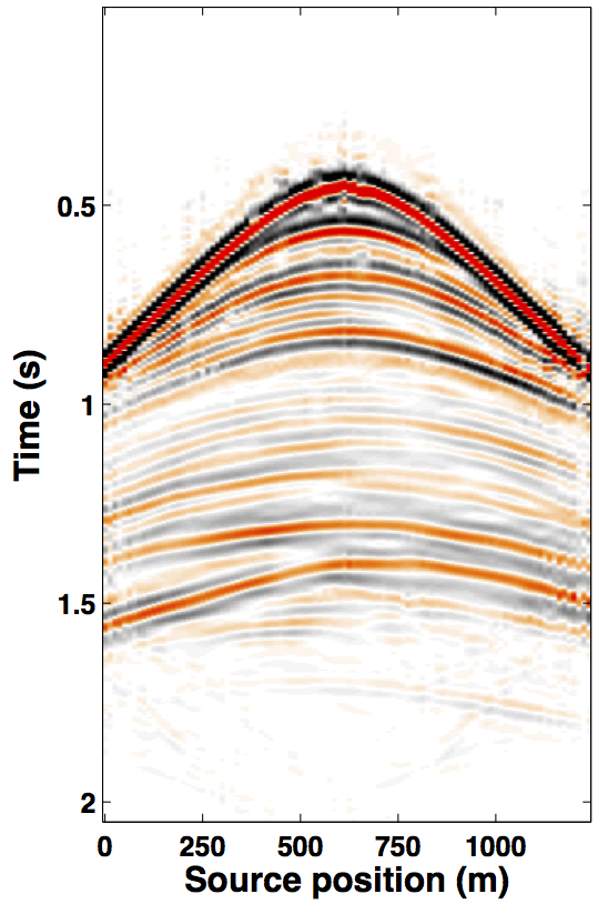
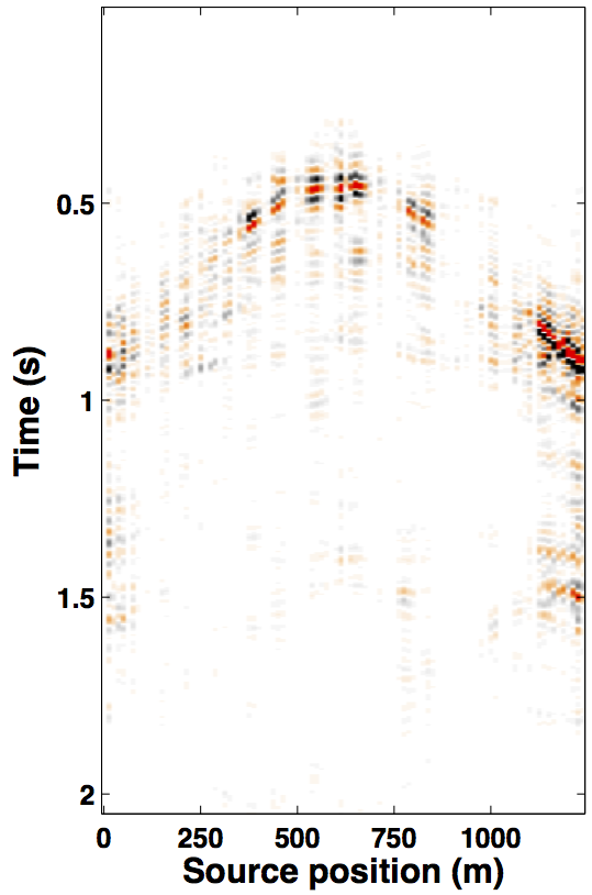
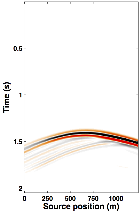
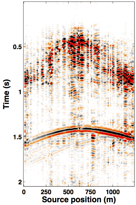
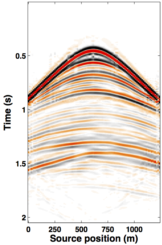
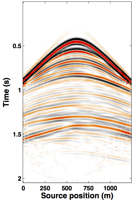
To illustrate the performance of our proposed JRM in the given situation of off-the-grid surveys where we can not exactly repeat, we simulate the off-the-grid (Figure 1) time-jittered baseline and monitor acquisitions on a synthetic 4-D dataset (same as used in Oghenekohwo et al. (2014)). With a source and receiver sampling of 12.5 m, the subsampling factor for the blended acquisition is 2. Since time-jittered acquisition results in a single long supershot of length \(n \leq N\), we (can) work with a single receiver (one trace of the supershot) incorporating all the jittered shots. Conventional time samples \(N_t = 512\) and shots \(N_s = 100\). In both the IRS and JRM, we recover the densely sampled data (from the subsampled, blended data) using a 2-D non-equispaced fast discrete curvelet transform (NFDCT, adapted from Hennenfent et al. (2010)) that handles irregular sampling, thus, exploring continuity along the wavefronts by viewing seismic data in a geometrically correct way—typically non-uniformly sampled along the spatial axes (source and/or receiver).

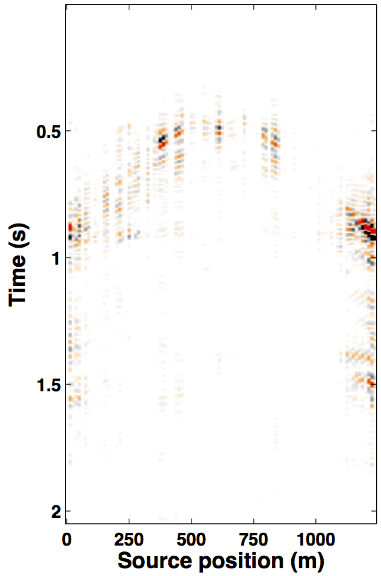
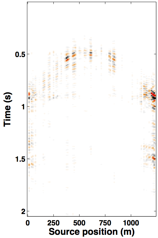
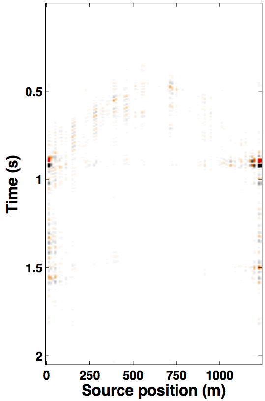
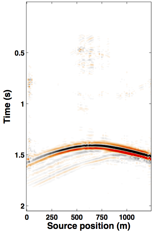
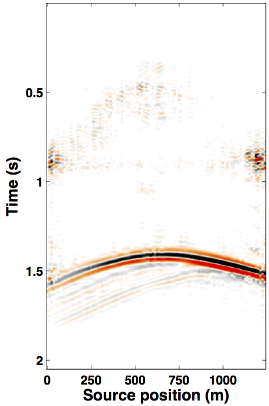
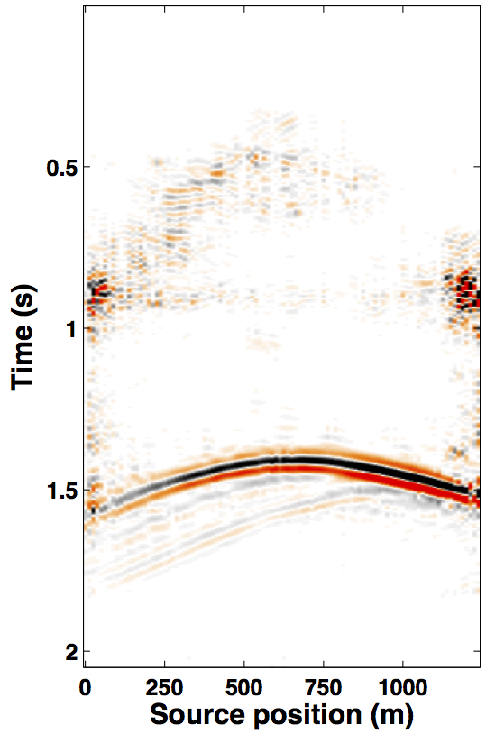
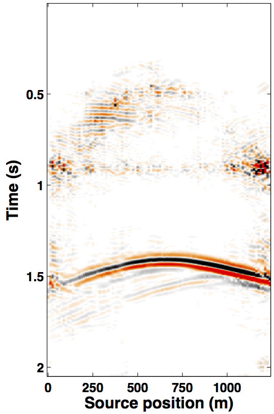
Due to limited space, we show recovery results for the monitor only, however, the observations for the baseline recovery are same. IRS and JRM recovered monitor data for \(50\%\) exactly repeated time-jittered acquisition (for the baseline and the monitor surveys) are shown in Figures 3a, 3b and Figures 4a, 4e, respectively. The corresponding IRS and JRM recovered 4-D signals are shown in Figures 3d and 4i, respectively. As illustrated, JRM performs better since it exploits the shared information between the two surveys. Henceforth, we only show the JRM results. The real world, however, suffers from calibration errors (Figure 1). As errors start to creep into the acquisition matrix, recovery of the 4-D signal deteriorates rapidly with increasing errors. Figures 4j, 4k illustrate this observation wherein errors as small as within 1.0 m adversely affect the 4-D signal recovery. As the error increases, 4-D signal recovery becomes comparable to the recovery with \(0\%\) overlap between the surveys (Figure 4l), which is inherent of randomized simultaneous acquisition (Figures 2b,2c). On the contrary, increasing calibration errors improve recovery of the vintages (Figures 4b, 4c, 4f, 4g), with \(0\%\) overlap giving the best recoveries (Figures 4d, 4h). Note that these recoveries are from incomplete acquisitions. Therefore, a dense baseline can not be used to generate data to compare with by applying the monitor (acquisition matrix) to the dense baseline since we also can not exactly repeat.

In conclusion, time-jittered blended marine acquisition can be extended to time-lapse surveys. Since, calibration errors are inevitable in the real world, and given the context of randomized subsampling, the requirement for repeatability in time-lapse surveys can be relaxed. Future work includes a detailed investigation of the effects of randomization and repeatability in time-laspe seismic while working with more realistic datasets.