Using common information in compressive time-lapse full-waveform inversion

Introduction

Full-waveform inversion (FWI) is a nonlinear problem that finds the model parameters that characterize the earth from measured seismic data (J. Virieux and Operto, 2009). Time-lapse seismic data can be used to provide information about changes in the subsurface over a period of time (Lumley, 2001). As an example, full-waveform inversion of time-lapse seismic data has been applied to storage and monitoring of \(\text{CO}_2\) (Queißer and Singh, 2013). While there have been a few attempts to apply FWI to time-lapse seismic data (Raknes et al., 2013; Asnaashari et al., 2014), some of the challenges of processing time-lapse data still persist. Issues such as differences in geometry, weak 4-D signals below the level of inversion or migration artifacts pose a challenge to the inversion algorithms (Lumley et al., 1997).

To address some of the challenges of processing time-lapse data, a few inversion methods (Shragge et al., 2013; Maharramov and Biondi, 2014) have been proposed. One common idea in these methods is to use a prior information in the baseline inversion for the monitor inversion. Another approach is a joint or simultaneous inversion of the baseline and monitor data. Both strategies are used in order to extract better time-lapse difference models that are obtained by subtracting the baseline and monitor inversion results. However, none of these methods explicitly use the shared information in the time-lapse data. In this work, we propose a noveau joint inversion algorithm where we exploit the shared information between the baseline and monitor data. Leveraging ideas from distributed compressed sensing (Baron et al., 2009), and stochastic optimization, we present an inversion framework that is fast, and gives a better time-lapse difference model compared to a similar independent or parallel inversion approach that doesn’t exploit the shared information in the data. Our algorithm combines our earlier work on joint recovery from subsampled time-lapse data (F. Oghenekohwo et al., 2014; Wason et al., 2014) and the modified Gauss-Newton inversion strategy proposed by Li et al. (2012). The efficacy of our proposed method is demonstrated on a realistic synthetic velocity model, which shows the imprint of a gas cloud in the time-lapse difference model.

Methodology

To arrive at an inversion formulation for time-lapse seismic data, we describe FWI on baseline (\(j = 1\)) and monitor (\(j = 2\)) data as the solution to the following problem: \[ \begin{equation} \label{eqfwitlapse} \tilde{\vector{m}_j}= \argmin_{\vector{m}_j}\|\vector{d}_j - \optensor{F}(\vector{m}_j)\|_2^2 \quad \quad \text{for}\quad j=\{1,2\}, \end{equation} \] where \(\optensor{F}\) represents the operator generating synthetic data from time-lapse model parameters \(\vector{m}\), and \(\vector{d}\) is the measured field data. In this formulation, \(\tilde{\vector{m}}_1\) and \(\tilde{\vector{m}}_2\) represent the final inversion results of the baseline and monitor, respectively. Constrained Gauss-Newton (GN) subproblems involve the pseudo-inverse of the reduced Hessian, computed from the Jacobian operator \(\nabla \optensor{F} (\vector{m}^k)\). The subproblems can be used to set up a GN update (\(\delta\vector{m}^k\)) for FWI at the \(k-\)th iteration. For time-lapse inversion, this translates to updates of the models via the following step: \[ \begin{equation} \label{eqfwistep} \vector{m}^{k+1}_{j} = \vector{m}^k_{j} + \delta\vector{m}^k_{j}. \end{equation} \] Li et al. (2012)] showed that the GN updates are sparse,-i.e. \(\delta\vector{m}_j = \vector{S}^H\vector{x}_j\); where \(\vector{S}^H\) is the conjugate transpose of a sparsifying transform \(\vector{S}\) and \(\vector{x}_j\) is a vector of transform coefficients. By linearizing the objective function of Equation \(\ref{eqfwitlapse}\) and promoting sparsity of the GN updates, the time-lapse FWI problem in Equation \(\ref{eqfwitlapse}\) becomes: \[ \begin{equation} \label{eqfwitlapse_sparsity} \tilde{\vector{x}}_j^k = \argmin_{\vector{x}_j} \frac{1}{2}\|\vector{d}_j^k - \optensor{F}(\vector{m}_j^k) - \nabla\optensor{F}(\vector{m}_j^k)\vector{S}^H\vector{x}_j\|_2^2 \quad \text{subject to}\ \|\vector{x}_j\|_1 < \tau_j^k \quad \text{for}\quad j=\{1,2\}. \end{equation} \] To choose \(\tau_j^k\), we follow the modified Gauss-Newton(mGN) strategy by Li et al. (2012). In fact, Equation \(\ref{eqfwitlapse_sparsity}\) gives parallel inversion results for the baseline and monitor data. Naively inverting for the baseline model and monitor model independently does not account for the shared information in the data. In our recent work (F. Oghenekohwo et al., 2014) on time-lapse seismic data recovery from subsampled data, we presented a joint recovery method (JRM) that exploits the shared information in the time-lapse vintages. Our method recovered time-lapse vintages and differences that are better than the estimates from parallel or independent processing. Incidentally, the mGN updates in Equation \(\ref{eqfwitlapse_sparsity}\) look very much like the problems we solve using the JRM. Therefore, this motivates the extension of the JRM to inversion of time-lapse seismic data.

Inversion with JRM

We consider two signals \(\vector{x}_1\) and \(\vector{x}_2\) representing the mGN updates for baseline and monitor inversion, respectively. These signals share a common component \(\vector{z}_0\) while each individual signal has an innovation component \(\vector{z}_j\). Therefore, each signal can be written as \[ \begin{equation} \label{eqjrm} \vector{x}_j = \vector{z}_0 + \vector{z}_j, \qquad j \in {1,2}. \end{equation} \] Using this model, we define for the \(k-\)th iteration of mGN for time-lapse FWI

\(\vector{b}^k = \begin{bmatrix} \vector{d}_1^k - \optensor{F}(\vector{m}_1^k) \\ \vector{d}_2^k - \optensor{F}(\vector{m}_2^k) \\ \end{bmatrix}, \quad \vector{A}^k = \begin{bmatrix} \nabla\optensor{F}(\vector{m}_1^k)\vector{S}^H & \nabla\optensor{F}(\vector{m}_1^k)\vector{S}^H & \tensor{0} \\ \nabla\optensor{F}(\vector{m}_2^k)\vector{S}^H & \tensor{0} & \nabla\optensor{F}(\vector{m}_2^k)\vector{S}^H \end{bmatrix}, \quad \vector{z}^k = \begin{bmatrix} \vector{z}_0^k \\ \vector{z}_1^k \\ \vector{z}_2^k \end{bmatrix}. \)

Contrary to the independent approach, which solves separate inversion problems for the vintages, without exploiting their correlations, the JRM exploits these correlations by solving one GN problem at the \(k-\)th iteration: \[ \begin{equation} \label{eqfwitlapse_jrm} \tilde{\vector{z}}^k = \argmin_{\vector{z}^k} \frac{1}{2}\|\vector{b}^k - \vector{A}^k\vector{z}^k\|_F^2 \quad \text{subject to}\ \|\vector{z}^k\|_1 < \tau^k. \ \end{equation} \] Equation \(\ref{eqfwitlapse_jrm}\) summarizes our proposed joint inversion scheme using the MGN algorithm. As stated previously, we refer to Li et al. (2012) regarding the selection of \(\tau^k\). The model updates from the above optimization problem for the baseline and monitor models are \[ \begin{equation} \label{eqjrm_update_} \vector{m}_j^{k+1} = \vector{m}_j^k + \vector{S}^H (\tilde{\vector{z}}_0^k + \tilde{\vector{z}}_j^k ). \end{equation} \] In the next section, we illustrate the performance of this method by means of a synthetic example that characterize realistic time-lapse scenarios.

BG Compass time-lapse model

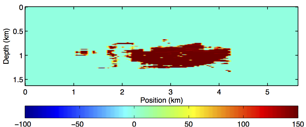
We study our formulation by means of synthetic experiments on the BG Compass time-lapse velocity model (Figure 1), showing the baseline, and the time-lapse difference anomaly obtained by subtracting the baseline and monitor (not shown). All the inversion results were obtained using a good initial model and the same starting model was used for the baseline and monitor inversion. All synthetic data are generated using a finite-difference acoustic modeling engine based on the constant density acoustic wave equation in the frequency domain. The range of velocities in the baseline and monitor models is between 1480m/s and 4500m/s (Figure 1a), while the time-lapse difference is plotted on a color scale of -100m/s to 150m/s. The inversion results are also displayed using the same color scale.

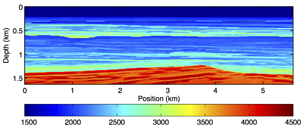
Using a Ricker wavelet with central frequency of 12Hz, 226 receivers sampled at 25m interval, and 112 shots sampled at 50m interval, a dense baseline data was generated. Two sets of dense monitor data were generated with similar receiver geometry. However, in the first set, the source acquisition geometry was exactly the same for the baseline but in the second set, same number of sequential shots were acquired by shifting the original source locations by 12.5m. This second monitor acquisition serves as a proxy for time-lapse data acquisition with non-repeated or inconsistent acquisition geometry.

The inversion procedure is based on a rerandomization procedure which entails the use of simultaneous shots as part of each mGN subproblem. The rerandomization corresponds to giving the sequentially sampled shots a different set of random weights at every step of the inversion. Details of this technique have been published by Li et al. (2012) and it’s beyond the scope of this work. The main idea is to use only a subset of the total data during every step of the inversion. This approach has been shown to reduce the computational cost required for the inversion and this efficiency motivates the adaptation of the method to our experiments on time-lapse FWI. Using simultaneous shots from the baseline and monitor data, we perform the independent or parallel inversion (Equation \(\ref{eqfwitlapse_sparsity}\)) and compare the results with the inversion with JRM (Equation \(\ref{eqfwitlapse_jrm}\)).

Experiments

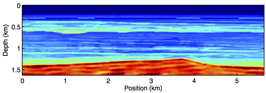
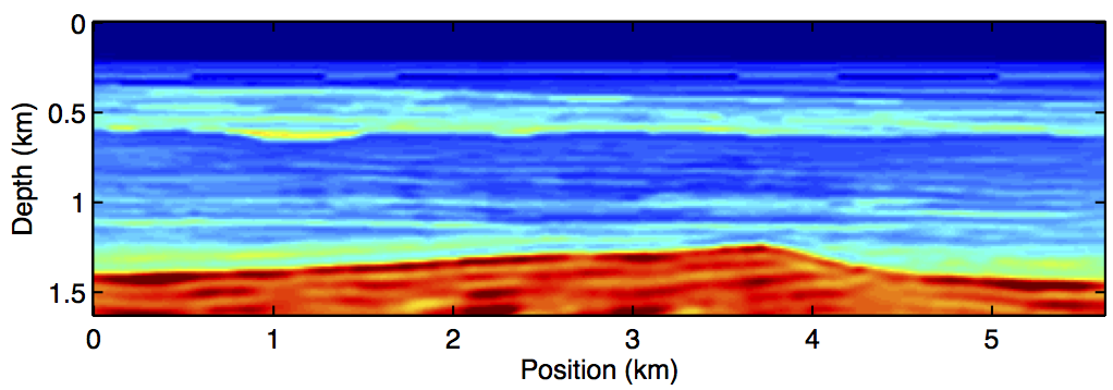
We conduct four experiments spanning the range of possible acquisition and processing scenario, namely, (i) Repeat acquisition and processing, (ii) Repeat acquisition with different processing, (iii) Different acquisition but same processing, (iv) Different acquisition with different processing. In these experiments, repeated processing means we are using the same random weights to generate the simultaneous shots. In all cases, we compare parallel inversion with joint inversion using JRM. We find, judging from the signal-to-noise ratio (SNR), that the third scenario gave the best time-lapse inversion results for the parallel (SNR = 4.4dB) and joint (SNR = 6.0dB) methods. Figure 2 shows the inversion results for the monitor and time-lapse signal in this scenario–i.e. different acquisition and same processing. In addition, we observe the results of inversion with JRM to be better than the parallel inversion in all the scenarios.

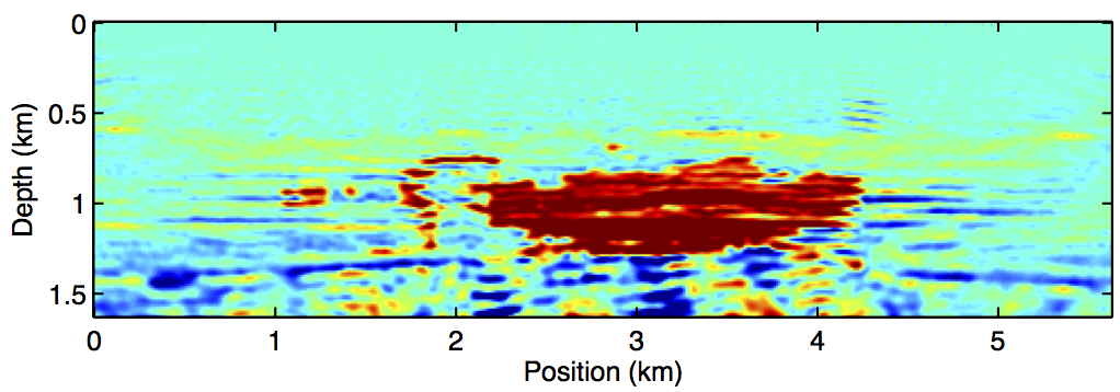
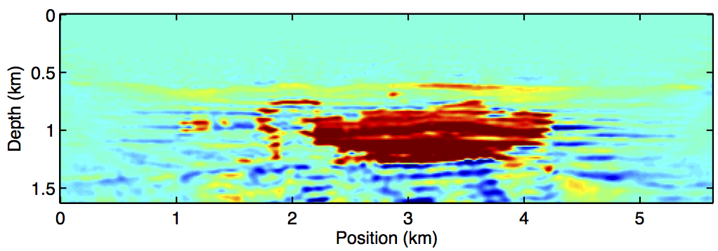
Discussion

The results we have shown indicate the benefits of our joint inversion algorithm over the independent or parallel inversion method. In both methods, we used a starting model close to the true baseline model in order to mitigate some common FWI problems such as local minima. We also used a common source signature for both inversions to reduce any repeatability effects in the data arising from different source functions. Although we expect our method to be able to address such effects in the data, that will be a subject of future research. Both the independent and joint FWI approaches were able to detect the time-lapse anomaly. However, we see less artifacts in the latter method (Figure 2d) compared to the former (Figure 2c). This improvement is due to the shared information between the baseline and monitor data, which the joint inversion method exploits but the independent inversion doesn’t. We also expect our observations to remain consistent in cases where the observed data is noisy since our method is able to handle non-sparse changes. Preliminary findings from our experiments further indicate that our joint inversion method is robust when time-lapse data is acquired with similar or different geometries. This further distinguishes our method from other inversion approaches that are based on a data difference idea, where the sources and receivers location must be exactly the same between the time-lapse surveys. More detailed comparison to other existing time-lapse inversion approaches will be the subject of future research.

Conclusions

We have presented a joint full-waveform inversion technique which is based on using the shared information between the baseline and monitor data. By using compressively sampled shots to speed up the inversion procedure, we find that our technique can significantly reduce time-lapse artifacts that mask true time-lapse signals. In addition, we have shown that our method is better than an independent inversion approach since it detects the true time-lapse anomaly while removing any unwanted artifacts.

Acknowledgements

We would like to thank BG Group for providing the time-lapse velocity model and all of the sponsors of our SINBAD project for their continued support.