Fast “online” migration with Compressive Sensing

Motivation

Wave-equation based migration corresponds to computing \[ \begin{equation} \label{eq:migration} \delta \vector{m}=\sum_{i=1}^K\nabla \vector{F}_i^\ast(\vector{m}_0,\vector{q}_i)\delta\vector{d}_i, \end{equation} \] where the sum runs over the number of experiments, indexed by \(i=1\cdots K\). For seismic applications, this number \(K\) is typically very large. These experiments—with sources \(\vector{q}_i\) and corresponding data \(\delta\vector{d}_i\)—involve either individual traces for different source/receiver pairs as in Kirchoff migration or (monochromatic) shot records as in (time-harmonic) reverse-time migration. In either case, the computational costs, including data-storage and movement, grows with \(K\) and the size of the survey area. To make matters worse, migration often relies on increasing the fold, to stack out unwanted artifacts in the image space, or on carrying out least-squares migration. In either case, the aforementioned increased costs strain even the largest computational resources stifling the adaptation of sparsity-promoting inversion techniques.

To overcome these costs, which are exacerbated by rapidly increasing costs of RTM as the frequency increases, we proposed randomized algorithms based on certain subsampling techniques that work on randomized subsets of the sources and corresponding data. These techniques have either lead to so-called batching techniques (Leeuwen and Herrmann, 2013a), where the above sum is approximated by carrying out the sum over subsets of randomly selected sources (or simultaneous sources), or to techniques based on Compressive Sensing (Herrmann and Li, 2012). Contrary to batching techniques, where the error is controlled by increasing the size of the subsets, sampling related errors during Compressive Imaging are controlled by promoting curvelet-domain sparsity. By incorporating rerandomization techniques from stochastic optimization into sparsity-promoting imaging, we arrived at an imaging technology that is able to carry out sparsity-promoting least-squares migration working on small subsets at the cumulative costs of roughly one RTM carried out over all data (Herrmann and Li, 2012; Tu and Herrmann, 2014).

While our Compressive Imaging technology is certainly promising, it relies on the combination of a sophisticated \(\ell_1\)-norm solver (SPGl1, E. van den Berg and Friedlander, 2008), rerandomizations, and warm starts. This makes the resulting algorithm complicated, and therefore difficult to implement on industry-scale problems. In addition, there is, aside from empirical observations, no formal proof what optimization problem this heuristic randomized approach actually solves. Below, we present a new highly flexible sparse inversion methodology that derives from a recently proposed sparse Kaczmarz solver for online problems in Compressive Sensing using linearized Bregman iterations (Lorenz et al., 2014). The resulting algorithm is relatively simple and suitable for online problems where measurements—read application of rows of the linearized modelling operator and therefore terms in the sum of Equation \(\ref{eq:migration}\)—take time and parallel resources to evaluate.

We organize our work as follows. First, we briefly state a simplified version of the algorithm undergirding our Compressive Imaging technology and juxtapose it with the proposed algorithm. Next, we compare the performance of the proposed algorithm on seismic imaging problems, followed by conclusions.

“Online” sparse solvers

We are interested in solving the following (partly) separable—i.e., we have access to individual rows as in trace-based migration or blocks of rows as in shot migration—linear inverse problems, where we aim to estimate the image \(\vector{x}\) from measurements \(\vector{b}\in\R^M\) given by \(\vector{b}=\vector{A}\vector{x}\), with \(\vector{x}\) sparse or compressible, and \(\vector{A}\in \R^{M\times N}\) tall—i.e., \(M\gg N\). This overdetermined problem is different from Compressive Sensing where \(M\ll N\) and could in principle by solved easily by inverting \(\vector{A}\) with least-squares or by simply applying the adjoint. Unfortunately, since we are dealing with problems where there are many rows of \(\vector{A}\) that are expensive to evaluate, we can not follow this approach and we have to resort to working on randomized pairs \(\{\vector{A}_i,\vector{b}_i\}\), made of randomly selected subsets of rows only—i.e., we only have access to \(\vector{A}_i\in\R^{m\times N}\) and \(\vector{b}_i\in\R^m\) with \(m\ll N \ll M\). Our aim is now to come up with an algorithm where the total amount of work, read the total number of rows participating in the inversion, is roughly the same as the total number of rows of the total system , or terms in the sum of Equation \(\eqref{eq:migration}\)—i.e., \(L=m\times n_{k}\sim M\) with \(n_k\) the number of iterations of the solver.

Solution by Randomized Iterative Shrinkage-Thresholding Algorithm (RISTA)

While many algorithms have been developed to solve the convex Basis Pursuit problem for underdetermined \(\tensor{A}\)’s with \(m\ll N\) \[ \begin{equation*} \mathrm{BP:}\quad\quad \minim_{\vector{x}} \|\vector{x}\|_1\quad\text{subject to}\quad \tensor{A}\vector{x}=\vector{b}, \end{equation*} \] its solution often requires too many iterations, and therefore evaluations of \(\tensor{A}\) and its adjoint \(\tensor{A}^\ast\), to make this a viable option for industrial problems, where the matrices are either very large or expensive to evaluate or both. To overcome this problem, the authors proposed a method to accelerate this type of algorithms using ideas from approximate message passing. The key idea of that approach was to “break” buildup of correlations between the model iterates, \(\vector{x}_k\), and the matrix \(\tensor{A}\) by drawing randomized pairs \(\{\vector{A}_k,\vector{b}_k\}\) for each iteration \(k\). This results in Algorithm 1, a randomized version of the Iterative Shrinkage-Thresholding Algorithm (ISTA,Yin et al. (2008);Beck and Teboulle (2009)). For a fixed pair \(\{\vector{A}_k,\vector{b}_k\}\) and appropriately chosen step length \(t_k\) and \(\lambda\rightarrow 0^+\) (read as \(\lambda\) goes to \(0\) from above), Algorithm 1 provably solves BP. While RISTA type algorithms—where techniques from stochastic gradients are combined with sparsity promotion—lead to fast and therefore practical algorithms, their performance hinges on choices for the threshold. Not only do small \(\lambda\)’s lead to slow convergence, there is also no general proof that Algorithm 1 solves BP when choosing different pairs \(\{\vector{A}_k,\vector{b}_k\}\) for each iteration. So the question is whether there exists an alternative iterative solver that makes few assumptions on \(\tensor{A}\) and that is capable of working with small randomized subsets of rows and that is relatively simple to implement.

Solution by Randomized Shrinkage-Thresholding Kaczmarz Algorithm with linearized Bregman (RISKA)

Consider the following slight modification—i.e. we replace line 3 of Algorithm 1 by \(\vector{z}_{k+1}=\vector{z}_k-t_k\vector{A}_k^\ast(\vector{A}_k\vector{x}_k-\vector{b}_k)\). We call this Solution by Randomized Shrinkage-Thresholding Kaczmarz Algorithm with linearized Bregman (RISKA,Yin et al. (2008)). According to recent work by Lorenz et al. (2014), this modified algorithm solves for step lengths, \(t_k=\frac{\|\vector{A}_k\vector{x}_k-\vector{b}_k\|^2}{\|\vector{A}_k^\ast(\vector{A}_k\vector{x}_k-\vector{b}_k\|^2}\), \[ \begin{equation*} \mathrm{KB:}\quad\quad \minim_{\vector{x}} \lambda\|\vector{x}\|_1+\frac{1}{2}\|\vector{x}\|_2^2\quad\text{subject to}\quad \tensor{A}\vector{x}=\vector{b}. \end{equation*} \] For large enough \(\lambda\) (Leeuwen and Herrmann, 2013b), RISKA provably converges to the solution of BP. While the modification w.r.t. RISTA is at first sight relatively minor, its implications are profound and manifold. First, compared to RISTA the inversion involves two iterates, namely \(\vector{z}_{k+1}\), which seeks to minimize the \(\ell_2\)-norm of the residual, and sparse model iterates \(\vector{x}_k\) obtained by soft thresholding \(\vector{z}_{k+1}\) with the threshold \(\lambda\). Contrary to RISTA, updates for the \(\vector{z}_k\)’s are calculated by subtracting gradients computed with respect to the sparse model iterate \(\vector{x}_k\). Third, the role of the threshold \(\lambda\) fundamentally changes. Within RISTA, the \(\lambda\) determines the projection of the model iterates on a \(\lambda\) dependent \(\ell_1\) ball. For a fixed \(\lambda\) the iterations without drawing new pairs \(\{\vector{A}_k,\vector{b}_k\}\) solve the unconstrained problem \(\min_{\vector{x}} \frac{1}{2}\|\tensor{A}\vector{x}-\vector{b}\|+\lambda\|\vector{x}\|_1\). By taking the limit \(\lambda\rightarrow 0^+\) these unconstrained problems solve BP. Unfortunately, small \(\lambda\) lead to slow convergence (Hennenfent et al., 2008). For large-scale problems this makes it necessary to devise ingenious cooling techniques where the \(\ell_1\)-norm constraint is gradually relaxed, e.g. by decreasing the \(\lambda\)’s as the algorithm progresses. This process allows components to enter into the solution slowly while bringing down the residual. Thresholding within RISKA, on the other hand, plays a completely different role since it balances \(\ell_1\)- and \(\ell_2\)-norms on the model. This means in a way that RISKA is “auto tuning”—i.e., when we choose \(\lambda\) too high, the \(\vector{x}_k\) will be zeros but not the \(\vector{z}_k\)’s. As \(k\) increases, the large entries—these are the first candidates to enter the solution—in \(\vector{z}_k\) will grow while the noisy crosstalk will become smaller if we chose to work with randomized \(\{\vector{A}_k,\vector{b}_k\}\)’s. After sufficient iterations, the number of which can be reduced by using intelligent step lengths, components will enter the solution. A too large \(\lambda\) for RISTA, on the other hand, would lead to zeros and would require a lowering of \(\lambda\). Finally, RISKA solves a constrained problem, i.e., the data is fitted exactly (this can be relaxed to different norms error balls (Lorenz et al., 2013)). This has the advantage that step lengths can be larger leading to a very fast but above all extremely simple algorithm that lends itself well to (i) work on (randomized) subsets of the data. Depending on the available computational resources, this gives us the freedom to choose, for a fixed number of passes through the rows \(L\), an optimal batch size \(m\) by trading of numbers of iterations and numbers of available nodes partaking in the inversion. For RTM this means that we can control the number of PDE solves while for trace-based migration this would limit the total number of source-receiver pairs touched by migration; (ii) implement RISKA in existing industrial settings as long as one has access to randomized subsets of data \(\vector{b}_k\), the Born modelling \(\tensor{A}_k\), and its adjoint migration \(\tensor{A}^*_k\). For RTM this means randomly selected shots or simultaneous shots while for Kirchhoff migration one should have access to randomized traces; (iii) select data and rows adaptively, e.g. according to the norm of the rows of \(\tensor{A}\) or condition number of block of rows as described in the literature (Strohmer and Vershynin, 2009; Needell and Tropp, 2014).

Examples

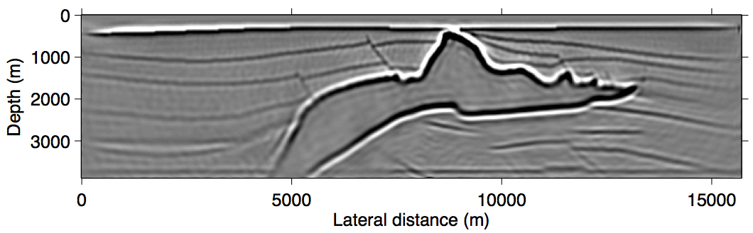
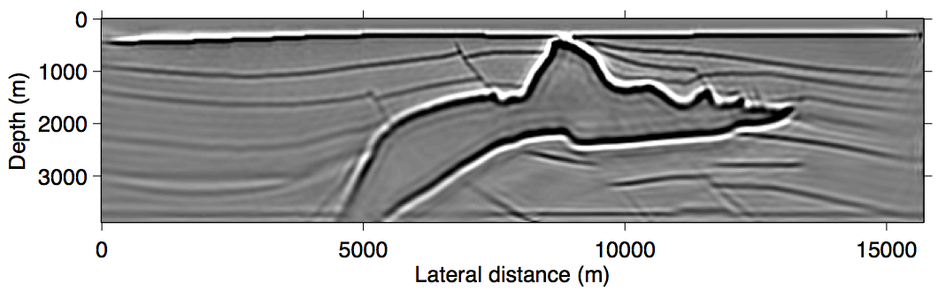
To illustrate the performance of RISKA, we compare sparsity-promoting linearized imaging results for primaries only and data including primaries and surface-related multiples obtained with our randomized SPGl1 solver and with the above described algorithm. In all examples, we fix the number of passes through the data to one (\(L=M\)), which are equivalent to the cost of a single RTM with all data. The results included in Figure 1 show improvements, especially below the Salt (juxtapose Figure 1a and 1b). These results are remarkable because we are able to obtain high-fidelity inversion results at the cost of a single RTM. An advantage of RISKA is that the underlying algorithm is simple to implement and relatively robust w.r.t. choices of \(\lambda\).

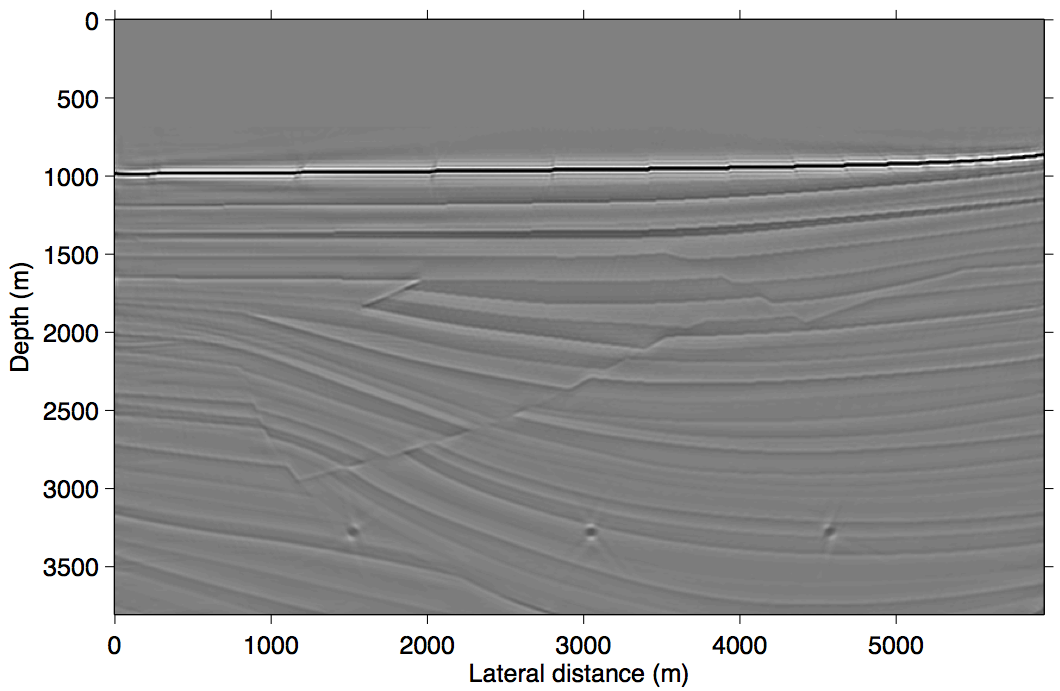
For the same budget (cost of 1 RTM), the proposed algorithm also produces improved results for an imaging example that includes surface-related multiples. In this case, we invert the linearized Born scattering operator with an areal source wavefield that contains the upgoing wavefield (Tu and Herrmann, 2014). Again, the results in Figure 2 are excellent despite the relative simplicity of the algorithm.

Conclusions

We presented a simplified randomized sparsity-promoting solver that provably converges to a mixed one- two-norm penalized solution while working on arbitrarily small subsets of data. This latter ability, in combination with its simplicity and “auto-tuning, makes this algorithm particular suitable for large-scale and parallel industrial applications.