Uncertainty quantification for Wavefield Reconstruction Inversion

Introduction

Full-waveform inversion (FWI) (Tarantola and Valette, 1982a; Virieux and Operto, 2009) is a popular method in seismic exploration that uses the waveform information to reconstruct subsurface structure. However, conventional FWI suffers from nonlinearity and local minima due to the elimination of the PDE constraint in the optimization problem. Wavefield reconstruction inversion (WRI) (Leeuwen and Herrmann, 2013; Peters et al., 2014) is a new approach of FWI that reduces the nonlinearity and lessens the effect of local minima. Instead of explicitly solving the wave equation, WRI relaxes the wave equation constraint by proposing a penalty formulation that explores both model and wavefield spaces. By exploiting this larger search space, WRI reduces the likelihood of reaching a local minimum. Moreover, compared to conventional FWI, whose Gauss-Newton Hessian is typically a dense matrix, the corresponding Gauss-Newton Hessian of WRI is a diagonal matrix and can be generated without any additional cost once wavefields are computed (Leeuwen and Herrmann, 2013).

Statistical inversion aims to obtain the posterior distribution of the model parameters given the distribution of the observed data and prior model information (Tarantola and Valette, 1982b) and quantify the uncertainty based on the posterior distribution. However, quantifying the uncertainty for conventional FWI is difficult. The forward mapping involves explicit PDE solves and is therefore very expensive computationally. Moreover the number of unknown parameters is also very large, which renders Markov chain Monte Carlo type methods intractable due to the large number of iterations needed to reach convergence. Moreover, due to the strong nonlinearity of the forward mapping, it is also difficult to generate an approximate distribution for the conventional FWI objective function to correctly quantify the uncertainty.

In this work, we propose a new posterior distribution, in which we use the wave equation misfit of WRI. Compared to the conventional FWI, the negative log-likelihood of this new posterior distribution is less prone to local minima and the Gauss-Newton Hessian, which is diagonal, is easy to obtain. These properties allow us to derive a Gaussian distribution that approximates the true posterior distribution, and quantify uncertainty based on this approximate distribution. No additional computational cost related to sampling and estimating the Gauss-Newton Hessian is required, unlike for the standard FWI case. This makes the method computationally feasible to quantify the uncertainty of WRI. Numerical experiments illustrate that the uncertainty quantified by this method is reasonable.

Posterior Distribution for WRI

The deterministic wavefield reconstruction inversion is aimed at solving the following unconstrained optimization problem \(\eqref{WRI}\), \[ \begin{equation} \label{WRI} \min_{\uvec,\vvec} \F(\uvec,\vvec)=\sum_{k,l}\|\Pmat_{k}\uvec_{k,l}-{\dvec}_{k,l}\|^{2}_{2} + \lambda^{2}\|\A_{k,l}(\vvec)\uvec_{k,l}-\q_{k,l}\|^{2}_{2}, \end{equation} \] which aims to balance the PDE misfit \(\A(\vvec)\uvec-\q\) with the data misfit \(\Pmat\uvec -\dvec\), simultaneously over velocity models \(\vvec\) and wavefields \(\uvec\), for all shots indexed by \(k = 1, 2, ..., N_{s}\) and a few relevant frequencies indexed by \(l = 1, 2, ..., N_f\). \(\Pmat\) is the operator that restricts wavefields to receiver locations, and \(\q\) represents sources. This joint optimization problem, as stated, is difficult to solve and requires a large amount of memory to store all the wavefields. One approach is to use the variable projection method (Leeuwen and Herrmann, 2013) to reduce the number of parameters by finding optimal wavefields \(\uvec\) for given velocity model \(\vvec\) at each iteration. As a result, the original joint optimization problem \(\eqref{WRI}\) is reduced to the problem \(\eqref{WRIvarprj}\), \[ \begin{equation} \label{WRIvarprj} \min_{\vvec} \F(\uvec(\vvec),\vvec)=\sum_{k,l}\|\Pmat_{k}\uvec_{k,l}(\vvec)-{\dvec}_{k,l}\|^{2}_{2} + \lambda^{2}\|\A_{k,l}(\vvec)\uvec_{k,l}(\vvec)-\q_{k,l}\|^{2}_{2}, \end{equation} \] and optimal wavefields \(\uvec\) are generated by solving the following least-squares problem \(\eqref{LSU}\): \[ \begin{equation} \label{LSU} \begin{split} \begin{pmatrix} \lambda{\A_{k,l}} \\ \Pmat_{k} \end{pmatrix}\uvec_{k,l} = \begin{pmatrix} \lambda{\q_{k,l}} \\ {\dvec}_{k,l} \end{pmatrix}. \end{split} \end{equation} \] In this work, we use the same idea from deterministic WRI to derive the posterior distribution of velocity models \(\vvec\) given observed data \(\dvec\) based on the Bayesian inference. The conventional statistical FWI defines the posterior distribution as the product of data misfit likelihood and prior distribution, which only considers the uncertainty of data. However, the forward modeling kernel also should contain uncertainty due to the fact that we do not fit the PDE exactly. Based on this observation, we derive a new posterior distribution of velocity models (Equation \(\ref{BayesianVARPRJ}\)), \[ \begin{equation} \label{BayesianVARPRJ} \rho_{\text{post}}(\vvec,\uvec(\vvec)) \propto \exp (- \sum_{k,l}\|\Pmat\uvec_{k,l}(\vvec) - {\dvec}_{k,l}\|^2_{\SIGMAN^{-1}} - \lambda^{2}\|\A_{k,l}(\vvec)\uvec_{k,l}(\vvec)-\q_{k,l}\|^{2}_{\SIGMAPDE^{-1}} - \|\vvec - \vvec_{\prior}\|^{2}_{\SIGMAP^{-1}}), \end{equation} \] which considers data misfit likelihood (the first term), wave equation misfit likelihood (the second term) and the prior distribution (the last term). Covariance matrices \(\SIGMAN\), \(\SIGMAPDE\) and \(\SIGMAP\) reflect uncertainty level and statistics of data, wave equation and prior model, respectively. We use variable projection method to generate optimal wavefields \(\uvec\) for fixed velocity model \(\vvec\) by solving the following least-squares problem \(\eqref{LSU2}\), \[ \begin{equation} \label{LSU2} \begin{split} \begin{pmatrix} \lambda\SIGMAPDE^{-1/2}{\A_{k,l}} \\ \SIGMAN^{-1/2}\Pmat_{k} \end{pmatrix} \uvec_{k,l} = \begin{pmatrix} \lambda\SIGMAPDE^{-1/2}\q_{k,l} \\ \SIGMAN^{-1/2}{\dvec}_{k,l} \end{pmatrix}. \end{split} \end{equation} \]

By involving the wave equation misfit, the Gauss-Newton Hessian of the negative log-likelihood of Equation \(\eqref{BayesianVARPRJ}\) is a diagonal matrix, which makes it less nonlinear than that of conventional statistical FWI (Leeuwen and Herrmann, 2013).

Quantify the Uncertainty

The posterior probability distribution \(\eqref{BayesianVARPRJ}\) is essential for the uncertainty quantification. However, quantifying statistical parameters based on Equation \(\eqref{BayesianVARPRJ}\) is extremely expensive because of the huge computational cost of solving least-squares problem \(\eqref{LSU2}\) and the high dimension of \(\vvec\). These properties renders traditional MCMC methods, which require an enormous amount of PDE solves (on the order of 10000 objective evaluations or more) in order to generate reasonable results, computationally intractable. An alternative method is to use a Gaussian distribution at the maximum likelihood point to approximate the original distribution, which is much cheaper to deal with than the posterior distribution (4).

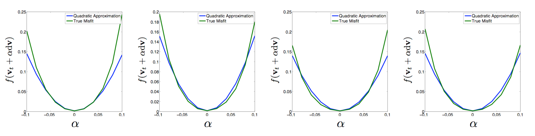
The approximate Gaussian distribution for conventional FWI is difficult to generate because the Gauss-Newton Hessian of the negative log-likelihood of the posterior distribution is dense and requires a large number of PDE solves to calculate. On the other hand, the Gauss-Newton Hessian of the negative log-likelihood of \(\eqref{BayesianVARPRJ}\) is a diagonal matrix. Using the following Equations (6) and (7), \[ \begin{equation} \label{WRIg} \g = \sum_{k,l}2\lambda^{2} \text{diag}(\text{conj}(\uvec_{k,l}))\frac{\partial{\A_{k,l}}}{\partial{\vvec}}^{T}\SIGMAPDE^{-1} (\A_{k,l}\uvec_{k,l}-\q_{k,l}), \end{equation} \] \[ \begin{equation} \label{WRIH} \Hmat = \sum_{k,l}2\lambda^{2} \text{diag}(\text{conj}(\uvec_{k,l}))\frac{\partial{\A_{k,l}}}{\partial{\vvec}}^{T}\SIGMAPDE^{-1} \frac{\partial{\A_{k,l}}}{\partial{\vvec}}\text{diag}(\uvec_{k,l}), \end{equation} \] we can compute the gradient and the diagonal Gauss-Newton Hessian and derive a quadratic approximation of the negative log-likelihood. Figure 1 shows the comparison of the negative log-likelihood (green line) and its quadratic approximation (blue line) at the maximum likelihood point (technically, the maximum a posteriori point or MAP) in four different random directions. We can observe that around the maximum likelihood point, the quadratic approximation matches the negative logarithm function quite well, which implies that the approximate Gaussian distribution \(\mathcal{N}(\vvec_{MAP}-\Hmat_{MAP}^{-1}\g_{MAP},\Hmat_{MAP}^{-1})\) is a good approximation to the posterior distribution.

Numerical Experiment

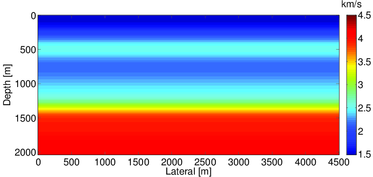
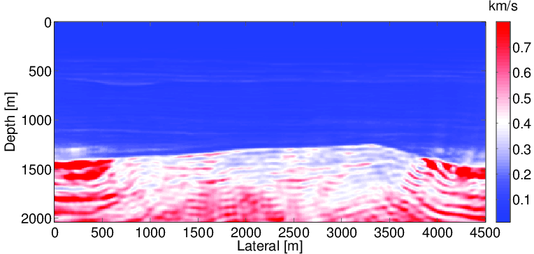
We test our uncertainty quantification method for WRI on the BG compass model. The model size is 4.5km x 2km. The true and initial models are shown in the Figure 2. 91 sources are located at the surface every 50m and 451 receivers are located at the surface every 10m. Ten frequency bands ranging from {2,3,4} Hz to {29,30,31} Hz are used for the inversion. In this experiment, to simplify the problem, we assume that we know the noise-free mean of the data, which may not be available in practice, and generate it using a 9-point finite difference method. The standard deviation for the noise of data is 1, the standard deviation for the PDE is 1 and the penalty parameter \(\lambda\) is selected to be 100 to balance the data misfit and PDE misfit. We assume that we do not have any prior information so that we do not include the prior distribution term in \(\eqref{BayesianVARPRJ}\) on our velocity models.

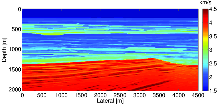
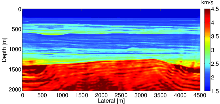
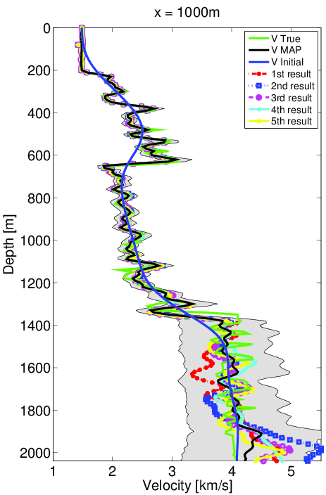
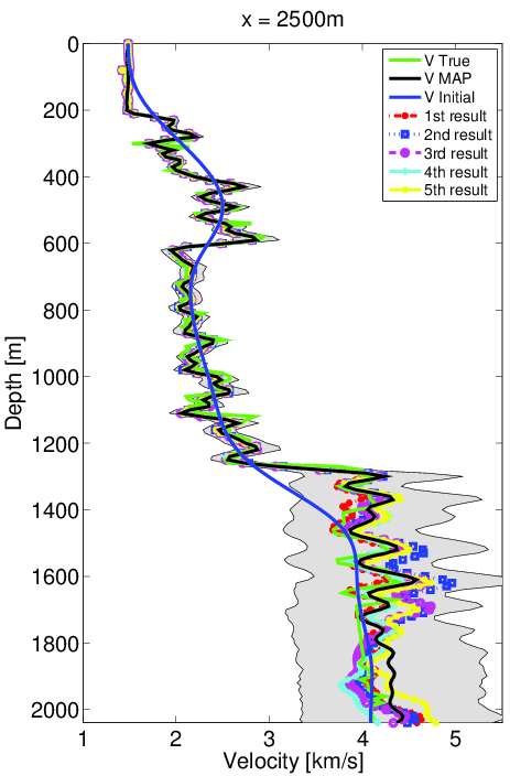
We first solve the deterministic optimization problem to find the maximum likelihood point (Figure 3a). Then we calculate the gradient and Gauss-Newton Hessian at this point and form the approximate Gaussian distribution. The standard deviation (Figure 3b) and confidence intervals (Figure 4) are computed using our Gaussian approximation to the true distribution. From the computed standard deviation, we observe that the standard deviation at the deep and boundary areas of the model is higher than in other areas, which agrees with our intuition. We also observe similar phenomena in the confidence interval results that the velocity in deeper regions has a larger uncertainty compared to shallower regions. Both observations corresponds to the fact that the observed data is less sensitive to the velocity in deep and boundary area.

In order to verify our uncertainty results, we invert five sets of data generated by adding noise according to the prescribed noise distribution above. These five results are shown in the Figure (4) with the initial model (blue line), true model (green line) and maximum likelihood point result (black line). All five of these results lie in the confidence interval, which indicates that our results are reasonable.

Conclusion

In this work, we propose a method to quantify the uncertainty of wavefield reconstruction inversion by introducing the wave equation misfit to the posterior distribution. This makes the negative log-likelihood of the posterior distribution less prone to local minima than in the FWI case and the diagonal Gauss-Newton Hessian is straightforward and efficient to generate. We use this Gauss-Newton Hessian to derive an approximate Gaussian distribution and quantify the uncertainty of the velocity model using this approximation. Since the Gauss-Newton Hessian is diagonal, we avoid solving a large number of PDEs that would otherwise have to be computed when estimating uncertainty for standard FWI. This method makes the uncertainty quantification for WRI computationally tractable and can provide reasonable uncertainty results based on the numerical experiments. In this work we assume we had noise-free data to compute confidence intervals as a proof of concept. In the future, we will consider the case of handling noisy data in our uncertainty quantification framework.

Acknowledgment

We thank all our sponsors of DNOISE II and SINBAD II for their continued support of this research..