Source Estimation for Wavefield Reconstruction Inversion

Introduction

Full-waveform inversion (FWI) is aimed at using the seismic signal to invert the subsurface structure by matching synthetic waveforms to observed waveforms (Tarantola and Valette, 1982; Virieux and Operto, 2009). Conventional FWI is susceptible to the so-called ‘cycle skipping’ problem that causes the local minima. Wavefield reconstruction inversion (WRI) (Leeuwen and Herrmann, 2013) is a new approach of waveform based inversion method that helps overcome this particular problem. Unlike the conventional FWI, which only explores the model spaces, WRI explores both model and wavefield spaces. With the larger search space, WRI is less likely to fall into local minima. Therefore it is able to start the inversion from higher frequencies and poorer initial models (Peters et al., 2014) compared to the conventional FWI.

Observed waveforms are dominated by the convolution of subsurface structure with source wavelets. Knowing source wavelets are essential for the waveform based inversion method, without correct source wavelets, wavefields cannot be reconstructed correctly and subsurface models cannot be inverted. It is well known that the variable projection method can be used to estimate source wavelets in the conventional setting of FWI (Li et al., 2013; Leeuwen et al., 2014; Aravkin et al., 2012), where it is only necessary to invert models and source wavelets jointly. Source estimation for WRI, on the other hands, is more difficult since wavefields are also unknowns.

In this work, we present a new source estimation method for WRI based on the variable projection method. In this method, we reconstruct wavefields and estimate source wavelets simultaneously by solving an extended least-squares problem. With these estimates, we update the subsurface model by a Newton type method. Numerical results illustrate that using our source estimation method we can recover source wavelets correctly and invert the velocity model even though we start from wrong source wavelets.

Source estimation for WRI

The conventional frequency domain full-waveform inversion inverts the subsurface velocity \(\v\) given the observed data \(\d\) by solving the following PDE-constrained optimization problem for all sources, indexed by \(k = [1,2,...,N_s]\), and a few relevant frequencies, indexed by \(l = [1,2,...,N_f]\) : \[ \begin{equation} \label{FWI} \begin{split} \minimize_{\u,\v}\sum_{k,l}\|\P_{k}\u_{k,l}-{\d}_{k,l}\|^{2}_{2} \\ \hspace{8mm} \text{ subject to } \A_{k,l}(\v)\u_{k,l} = \q_{k,l}, \end{split} \end{equation} \] where \(\A_{k,l}\) represents the Helmholtz matrix, \(\q_{k,l}\) is source function, and \(\P_{k}\) is the projection operator that restricts wavefields to receiver locations. The conventional approach to solve \(\eqref{FWI}\) is to eliminate the constraints by solving the wave equation explicitly, yielding the following reduced problem: \[ \begin{equation} \label{FWI2} \minimize_{\v}\sum_{k,l}\|\P_{k}\A_{k,l}(\v)^{-1}\q_{k,l}-{\d}_{k,l}\|^{2}_{2}. \end{equation} \] Empirically, solving the reduced problem \(\eqref{FWI2}\) tends to stuck in the local minima if starting from a poor initial model (Virieux and Operto, 2009).

Unlike the conventional approach eliminating wavefields by solving PDEs explicitly, WRI expands the search space and optimizes for both wavefields and velocities by solving the following penalty formulation of the constrained problem (Leeuwen and Herrmann, 2013): \[ \begin{equation} \label{WRI} \minimize_{\u,\v} \sum_{k,l}\|\P_{k}\u_{k,l}-{\d}_{k,l}\|^{2}_{2} + \lambda^{2}\|\A_{k,l}(\v)\u_{k,l}-\q_{k,l}\|^{2}_{2}. \end{equation} \] As demonstrated by Leeuwen and Herrmann (2013), the problem \(\eqref{WRI}\) can be solved by the variable projection method. Contrary to the conventional FWI, both wavefields and square of the slowness appear linearly in the problem \(\eqref{WRI}\). This implies that for every choice of velocity \(\v\), the optimal value for wavefields \(\u\) can be found by solving the following linear least-squares problem: \[ \begin{equation} \label{lsWRI} \begin{split} \begin{pmatrix} \lambda{\A_{k,l}} \\ \P_{k} \end{pmatrix}\u_{k,l} = \begin{pmatrix} \lambda{\q_{k,l}} \\ {\d}_{k,l} \end{pmatrix}. \end{split} \end{equation} \] Once the data-augmented system \(\eqref{lsWRI}\) is solved, the gradient and diagonal Gauss-Newton Hessian can be generated straightforwardly without additional computational cost (Leeuwen and Herrmann, 2013). On the contrary, the conventional FWI requires adjoint wavefields to generate the gradient and more PDE solves to generate the Gauss-Newton Hessian. We can use the gradient and Gauss-Newton Hessian to update the velocity model by a Newton type method.

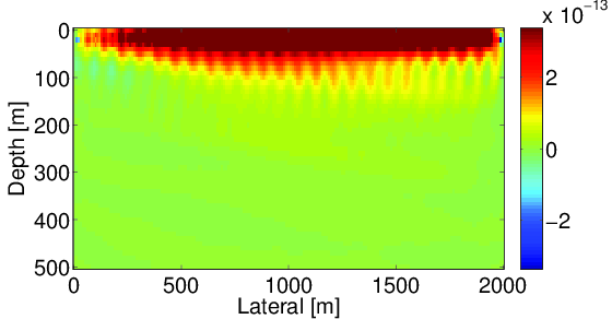
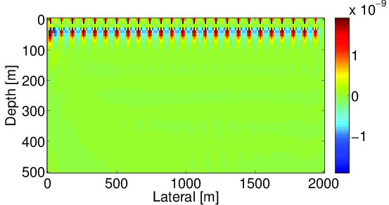
In our previous discussion, we assumed source wavelets were known. However, in most practical situations, true source wavelets are not available and must be estimated. Without correct source wavelets, reconstructed wavefields from Equation \(\eqref{lsWRI}\) will have a significant error compared to the true wavefields, which will result in a big difference in the gradient. In order to illustrate the importance of source wavelets, we include Figure 1 that shows the comparison of gradients using correct source wavelets and wrong source wavelets on a simple model. Comparing Figure (1a) and Figure (1b), we can observe that using wrong source wavelets, strong artifacts will arise around source positions. These artifacts destroy the gradient and will cause the inversion to fail very quickly.

Since modeling the source corresponds to a simple scaling, we can recast Equation \(\eqref{WRI}\) in the form of the following optimization problem: \[ \begin{equation} \label{WRIsrc} \minimize_{\u,\v, \alpha} \sum_{k,l}\|\P_{k}\u_{k,l}-{\d}_{k,l}\|^{2}_{2} + \lambda^{2}\|\A_{k,l}(\v)\u_{k,l}-\alpha_{k,l}\mathbf{e}_{k,l}\|^{2}_{2}. \end{equation} \] For \(k^{\text{th}}\) source and \(l^{\text{th}}\) frequency component, \(\alpha_{k,l}\) is the source wavelet and \(\mathbf{e}_{k,l}\) is a unit vector with nonzero element at the source location. Although three unknown parameters are involved in Equation \(\eqref{WRIsrc}\), we still can use the variable projection method to solve it by introducing a new parameter \(\x_{k,l} = [\u_{k,l}, \alpha_{k,l}]\), and transforming the original problem to a two-variable optimization problem. Fortunately, the new parameter \(\x\) appears linearly in the problem \(\eqref{WRIsrc}\), which allows us to use variable projection to solve it. For every choice of velocity \(\v\), optimal value for \(\x\) can be found by solving the following least-squares problem: \[ \begin{equation} \label{varprjsrc} \begin{aligned} \begin{pmatrix} \lambda{\A_{k,l}} & -\lambda{\mathbf{e}_{k,l}} \\ \P_{k} & 0 \end{pmatrix} \x_{k,l} = \begin{pmatrix} 0 \\ {\d}_{k,l} \end{pmatrix} \Longrightarrow \begin{pmatrix} \lambda{\A_{k,l}} & -\lambda{\mathbf{e}_{k,l}} \\ \P_{k} & 0 \end{pmatrix} \begin{pmatrix} \u_{k,l} \\ \alpha_{k,l} \end{pmatrix} = \begin{pmatrix} 0 \\ {\d}_{k,l} \end{pmatrix}. \end{aligned} \end{equation} \] Comparing problem \(\eqref{varprjsrc}\) and \(\eqref{lsWRI}\), the new data augment system \(\eqref{varprjsrc}\) is only one column larger than the original system \(\eqref{lsWRI}\). Therefore, no significant computational cost is required if a direct solver is used. Since the receiver positions are different, all columns of the projection operator \(\P_{k}\) are independent. Therefore, no nontrivial linear combinations of columns of \(\P_{k}\) are available to represent the zero vector, which indicates that columns of the new data augment system \(\eqref{varprjsrc}\) are independent and the new system has a unique least-squares solution.

As a result, for each source and each frequency, we reconstruct wavefields and scale the corresponding source wavelet simultaneously. This approach is better than alternating optimization of \(\u\), \(\alpha\) and \(\v\) , which does not guarantee convergence. With estimated wavefields and source wavelets, we can use the same Newton type method mentioned in previous paragraph to update the velocity model \(\v\).

Numerical Example

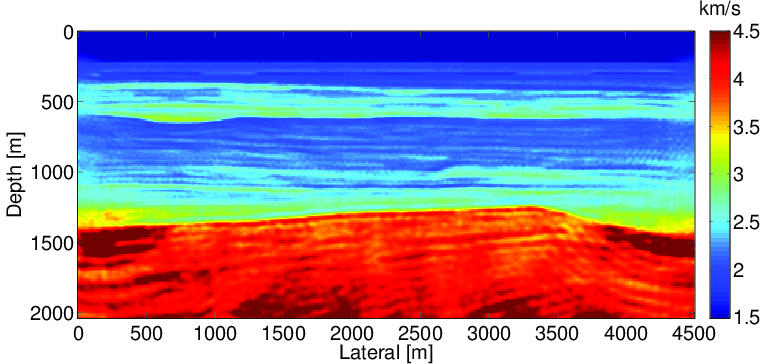
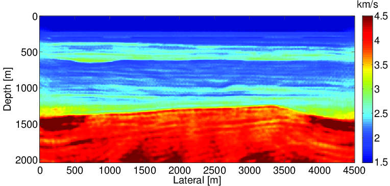
In this section, we test our source estimation method for WRI on the BG compass model. The model size is 4.5 km x 2.0 km. The true velocity is shown in the Figure 2a. The initial model (Figure 2b) is generated by smoothing the original model followed by a horizontal stacking. The source wavelet used is a Ricker wavelet with central frequency at 20 Hz. Ninety-one sources are located at the surface at 50m intervals, and 451 receivers are located at the surface at 10m intervals. Ten frequency bands ranging from {2,3,4} Hz to {29,30,31} Hz are used to invert the velocity. We assume that we do not have any information about the source wavelet, so the initial source wavelet we use is a simple spike pulse. In the inversion, we estimate the source wavelet shot by shot.

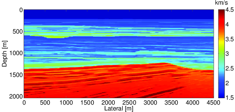
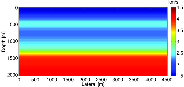
Figure 3 shows the comparison of first gradients we obtain using the true source wavelet (a), estimated source wavelet (b) and wrong source wavelet (c), respectively. From the comparison we can observe that using wrong source wavelets, the gradient has a significant difference from the true gradient with correct source wavelets. In the wrong gradient (c), the energy focuses around source positions due to the wrong source wavelets, while in the true gradient (a), the energy spreads to the shallow part of the model. On the other hand, unlike the wrong gradient (c), the energy of the gradient with estimated source wavelets (b) also spreads to the shallow part and is much closer to the one with correct source wavelets (a). This implies that our source estimation method can correct wrong source wavelets and help to improve the inversion.

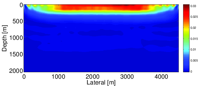
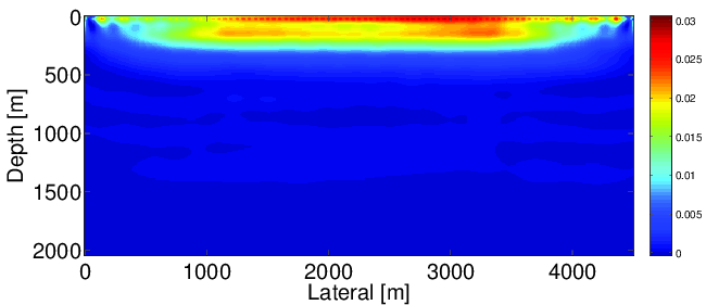
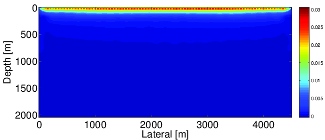
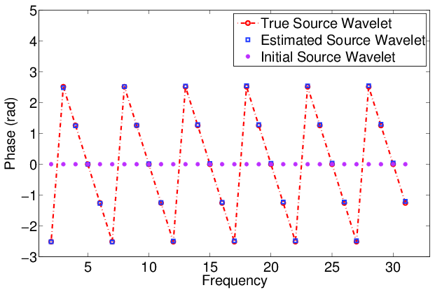
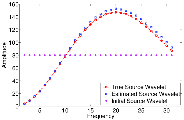
Figure 4 shows the comparison of inversion results obtained with correct source wavelets and estimated source wavelets. Only some slight differences at the deep part and boundary of the model can be observed. Figure 5 shows the comparison of the true source wavelet (red), estimated source wavelet (blue) and initial source wavelet (magenta). Both phase and amplitude are accurately recovered. There is only a small amplitude difference at high frequencies.

Conclusion

In this work, we use a variable projection method to propose a new method to estimate source wavelets for wavefield reconstruction inversion. Since both wavefileds and their corresponding source wavelets appear linearly in the WRI objective, we are able to reconstruct wavefields and estimate source wavelets simultaneously during the inversion procedure. Numerical experiments illustrate that using our source estimation method, we can recover source wavelets and obtain similar inversion result as from correct source wavelets. This demonstrates the feasibility of our method.

Acknowledgment

This work was in part financially supported by the Natural Sciences and Engineering Research Council of Canada Discovery Grant (22R81254) and the Collaborative Research and Development Grant DNOISE II (375142-08). This research was carried out as part of the SINBAD II project with support from the following organizations: BG Group, BGP, CGG, Chevron, ConocoPhillips, ION, Petrobras, PGS, Statoil, Total SA, Sub Salt Solutions, WesternGeco, and Woodside.