Off the grid tensor completion for seismic data interpolation

Curt Da Silva and Felix J. Herrmann
Seismic Laboratory for Imaging and Modeling (SLIM), The University of British Columbia

Introduction

A large amount of the effort in seismic data acquisition is dedicated to designing experiments that exactly conform to strict Shannon sampling theory. Data collected according to this theory must be sampled at or above the Nyquist rate and must conform to a regularly-spaced grid in order to avoid introducing aliasing and spurious artifacts. These requirements are often unable to be met in practice, due to uncontrollable forces affecting acquisition boats such as the shifting of oceanic waves. Owing to the high dimensionality of seismic data, the number of samples required by traditional Nyquist-based sampling is also large, which introduces further challenges to collect, store, and process such a volume.

Fortunately, despite its large size and high dimensionality, seismic data can be well represented as a low rank tensor, which allows us to represent the full data volume using much fewer parameters than the ambient dimension size. More importantly, this low dimensionality allows us to perform tensor completion on a seismic data volume with missing entries. By reducing the necessary number of samples acquired in the field, and subsequently the time and budget costs associated with acquisition, we can instead formulate a sampling scheme that allows us to solve an associated optimization problem to recover our full data. It is particularly important during a time of low oil prices to establish an acquisition paradigm that is cost-efficient. The theory of matrix completion, upon which tensor completion is built, stipulates that the subsampling operators should slow the singular value decay of the true signal in order for rank-minimizing recovery to work effectively.

In this abstract, we extend our previous work in tensor completion for seismic data volumes in Da Silva and Herrmann (2013) to handle seismic data acquired on an irregularly sampled grid, which we will refer to as ‘off-the-grid’ in this work. We will first briefly review the Hierarchical Tucker format and then develop our understanding of the challenges of off-the-grid tensor completion in terms of the singular values of different matricizations of seismic data, that is to say, reshapings of the seismic data volume in to matrices along various dimensions. Irregular, off-the-grid sampling destroys the low-rank structure of seismic data and we introduce an operator that resamples from a regular grid to the irregular acquisition grid to restore this low-rank behaviour. We refer to this operator as our regularization operator in this context. Using this approach, we solve a standard tensor completion problem and obtain significantly improved results compared to simply interpolating the binned data.

This work builds upon the ideas of off-the-grid regularized matrix completion for seismic data with missing traces in Kumar et al. (2014) and extends the regularization approach to the 3D data case. Other approaches to regularized interpolation include the Antileakage Fourier Transform (AFT) in Xu et al. (2005), Interpolated Compressed Sensing (ICS) in Li et al. (2012), and Non-uniform Curvelets (NCT) in Hennenfent et al. (2010). AFT reconstructs the largest, off-the-grid Fourier coefficients using Orthogonal Matching Pursuit, estimating a single component of the spectrum at a time. Aside from the lack of convergence guarantees, this method can lead to poor convergence if the underlying vector is not exactly sparse but has many quickly decaying coefficients, as is typical for real-world data. The ICS method introduces a polynomial regularization operator in to a traditional analysis Compressed Sensing problem, but employs a first order solver, which may converge slowly. The NCT approach has shown to be quite successful for 2D data sets, but the computational cost of curvelets limits its applicability to large 3D data sets.

Hierarchical Tucker Format

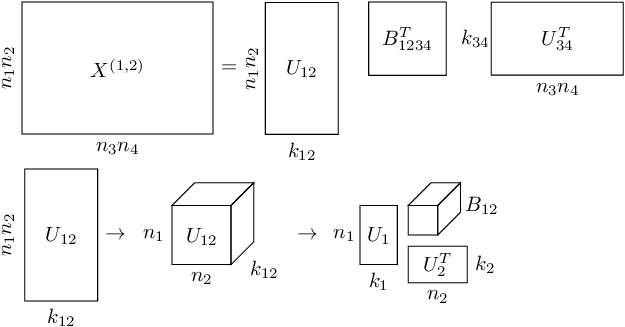
Given that the Hierarchical Tucker tensor format is relatively unknown and not widely used, we detail some of its construction here. One of the key operations on tensors is that of matricization.

Definition The matricization of a \(d-\)dimensional tensor \(\mathbf{X}\) along the modes \(t \subset \{1, 2, \dots, d\}\) is the matrix, denoted \(X^{(t)}\), is the reshaping of \(\mathbf{X}\) in to a matrix with the dimensions specified by \(t\) being vectorized along the rows and the remaining dimensions are vectorized along the columns. For example, \(X^{(1)}\) places the first dimension along the rows and the \(2,3,4\) dimensions along the columns.

The Hierarchical Tucker (HT) tensor format is summarized pictorially in Figure 1. For say, a 4D frequency slice of data \(\mathbf{X}\), with dimensions \(n_1 \times n_2 \times n_3 \times n_4\), we reshape it in to a matrix \(X^{(1,2)}\) with the first two dimensions along the rows and the last two dimensions along the columns. We stipulate an “SVD-like” decomposition on this matrix \(X^{(1,2)}\) to obtain the matrices \(U_{12}, B_{1234},\) and \(U_{34}\). In this way, we are ‘splitting apart’ the first two dimensions from the last two dimensions. We can further continue this splitting by reshaping \(U_{12}\) in to a 3D cube and performing an analogous decomposition between dimensions 1 and 2, as shown in the bottom of Figure 1. We apply the same splitting for \(U_{34}\).

This construction allows us to avoid having to store the intermediate matrices \(U_{12}, U_{34}\) explicitly, since the small matrices \(U_i\), \(i=1,2,\dots, 4\) and the small, intermediate tensors \(B_t\) specify the data \(\mathbf{X}\) completely. The number of parameters needed to parametrize HT tensors is \(\le dNK + (d-2)K^3 + K^2\), where \(N\) is the maximum individual dimension size, \(K\) is the maximum internal rank parameter, and \(d\) is the number of dimensions. For high dimensional volumes with \(K \ll N\), this quantity is much less than \(N^d\), the traditional storage requirements needed to store a \(d-\)dimensional tensor. This construction allows us to effectively break the curse of dimensionality for data volumes that exhibit this low-rank behaviour.

For seismic problems, we arrange \(X\) according to the coordinates \((x_{\text{src}},x_{\text{rec}},y_{\text{src}},y_{\text{rec}})\). This permutation promotes the decay of singular values in all dimensions, which allows it to be well-represented as a HT tensor . Due to source-receiver reciprocity, we assume for definiteness that our data is missing random receivers and we seek to interpolate it at these locations.

We formulate our interpolation problem in the HT format as follows. Given a receiver subsampling operator \(\mathcal{A}\) and a set of measurements \(b\), the optimization problem we solve to interpolate our data with missing traces is \[ \begin{equation} \label{optproblem} \min_{x = (U_t,B_t)} \|\mathcal{A} \phi(x) - b\|_2^2, \end{equation} \] where \(\phi(x)\) is the function that expands the small HT parameters \(x = (U_t, B_t)\) in to the full tensor space. We use our previous code in Da Silva and Herrmann (2014) for solving this problem and omit the specific details here due to space constraints. It suffices to say that we can solve this problem in an efficient manner, while avoiding the computation of SVDs of large scale matrices.

Singular values and regularization

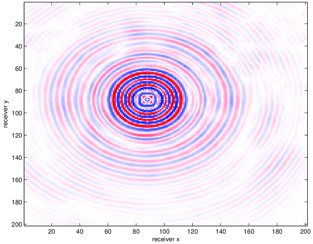
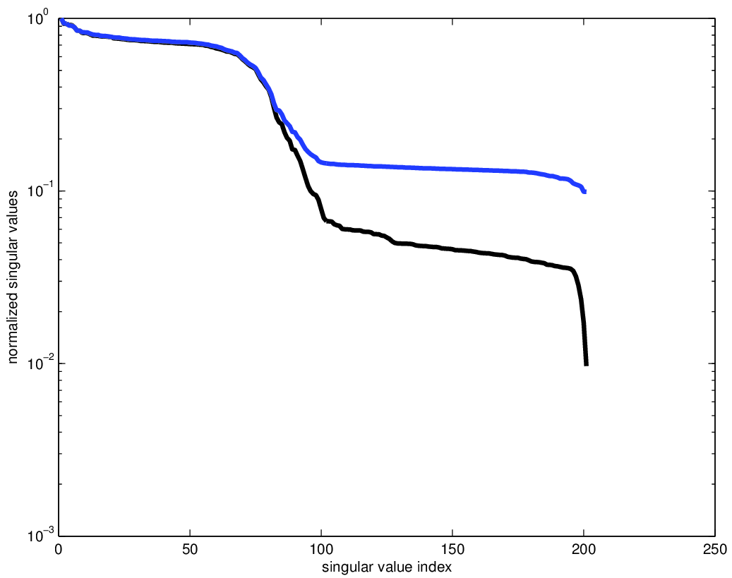
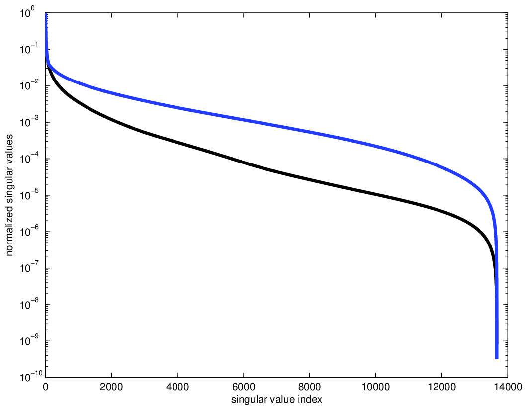
For our examples, we use a data set provided to us by the BG Group. The data volume has \(68 \times 68\) sources sampled on a 150m grid and \(401 \times 401\) receivers sampled on a 50m grid, from which we extract a temporal frequency slice at 7.34Hz. A seismic data volume can be well represented in the HT format precisely when the singular values of the various matricizations decay quickly. In order to understand the effect of on grid versus off grid subsampling, we regularly and irregularly subsample this volume in the receiver coordinates to a 100m spaced grid. For the irregular sampling, 50% of the samples are randomly perturbed off the regular 100m grid points to a point 50m away, as shown in Figure 2. We use this approach to avoid having to generate inverse crime data by an alternative interpolation method. We show the singular values of the matricizations along the \(x_{\text{src}}\), \(x_{\text{rec}}\), and (\(x_{\text{src}}\), \(x_{\text{rec}}\)) dimensions for both volumes in Figure 2. The original, regularly sampled data volume has singular values that decay much more quickly than its irregularly sampled counterpart. This indicates that the data volume is inherent not low rank for irregularly sampled data, and thus low-rank interpolation will not perform well. This sampling can also be considered as a binning approach, which is known to introduce large errors depending on the distance to an on-grid point, and is thus unsuitable for low rank interpolation.

In order to overcome this high-rank limitation of off-the-grid sampling, we introduce a fictious, regular grid in which the seismic data volume is low rank and an operator that interpolates from this regular grid to the irregular acquisition grid. We choose the Non-uniform Fourier Transform (NFT), although other choices are possible. In order to fit this operator in to our problem \(\eqref{optproblem}\), we replace our receiver subsampling operator \(\mathcal{A}\) with a new operator \(\widetilde{\mathcal{A}} = \mathcal{A} P^T ( N \otimes I_{n_s^2} ) P\). Here \(P\) permutes the coordinates of the tensor from \((x_{\text{src}},x_{\text{rec}},y_{\text{src}},y_{\text{rec}})\) (the low-rank ordering) to \((x_{\text{src}},y_{\text{src}},x_{\text{rec}},y_{\text{rec}})\) (the standard ordering) and \(P^T\) is its adjoint, which reverses the permutation. \(N\) is the NFT operator that interpolates from a uniform spatial frequency grid to the irregular spatial sampling grid in the receiver coordinates and \(I_{n_s^2}\) is the identity operator in the source coordinates.

By simply initializing our problem with this new operator \(\widetilde{\mathcal{A}}\), we can reuse our previous code for regularly-spaced HT completion with minimal changes. The primary costs of our algorithm are now the application of the NFT operator across the receiver coordinates. In our experiments, this choice of regularization operator gave much better results than mere linear or cubic interpolation, which were faster to apply. In practical applications, it is important to choose an operator that balances the tradeoff between reconstruction quality and speed of application. Owing to the fact that our HT optimization algorithms converge quickly (typically in 15-20 iterations), we only need to apply our regularization operator a minimal number of times.

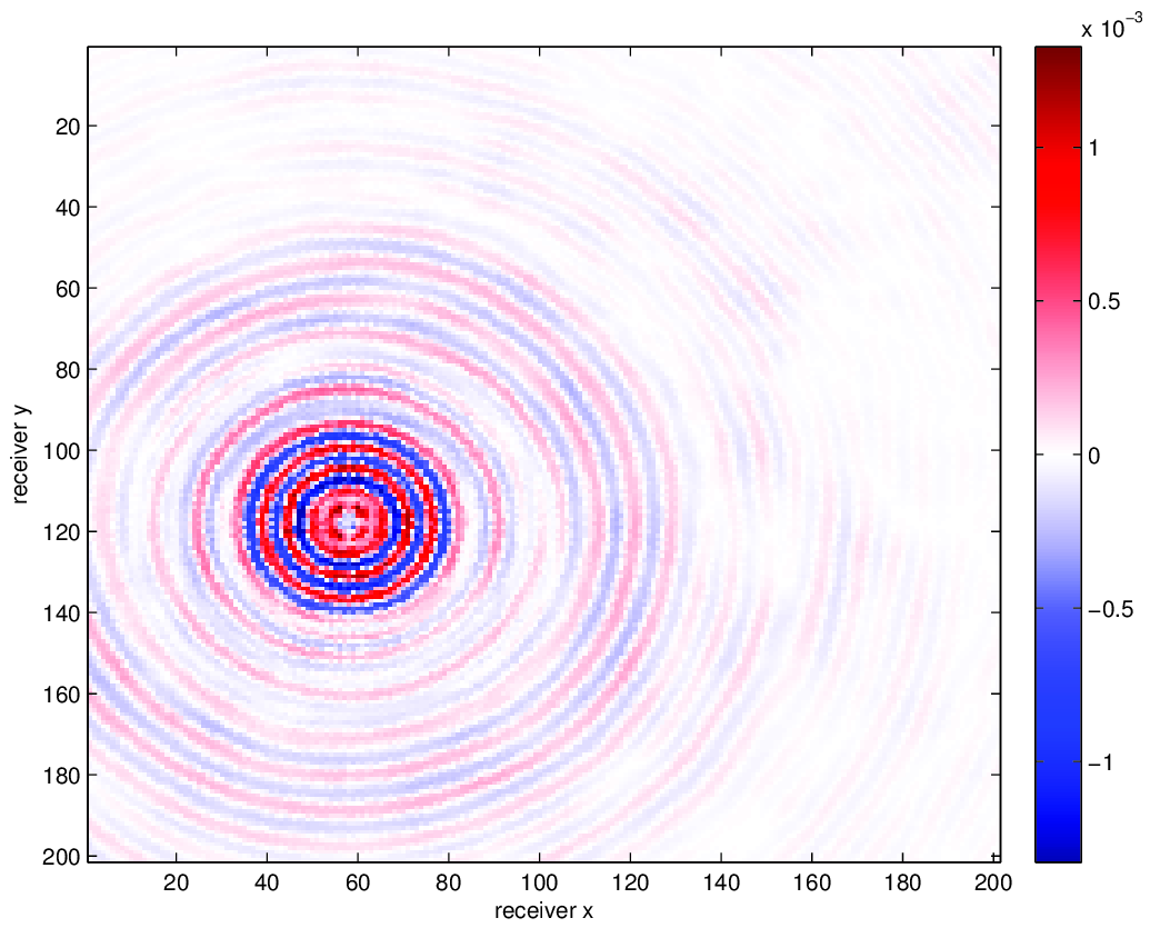
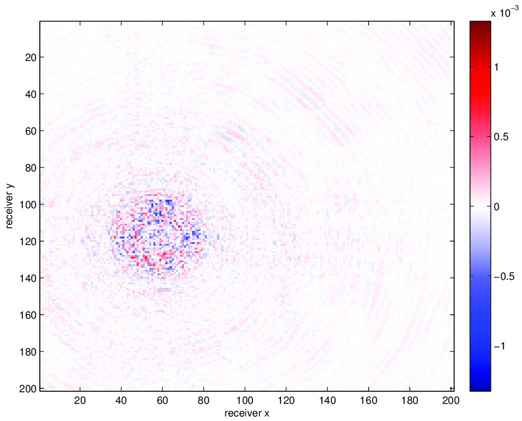
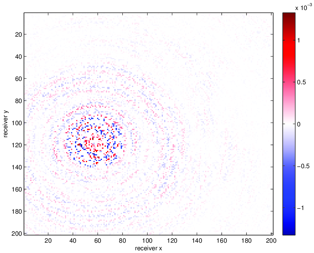
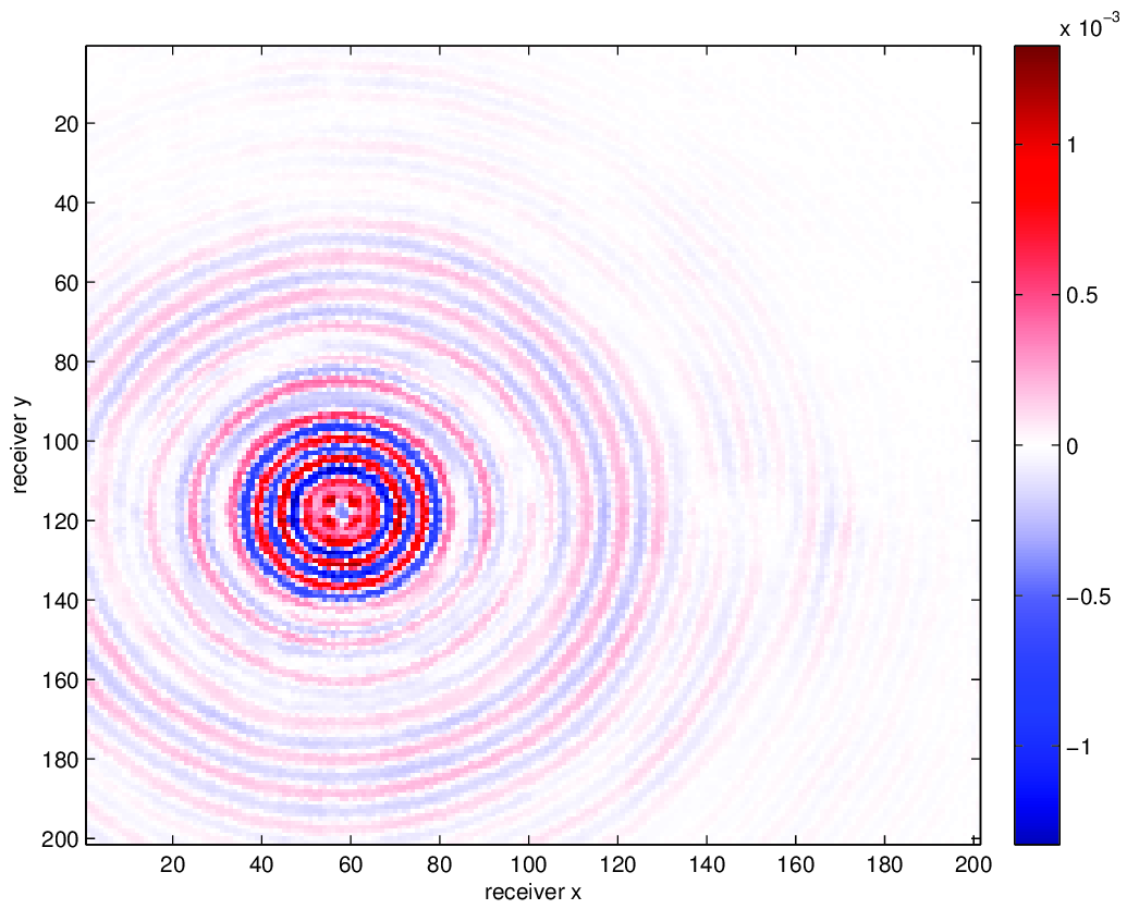
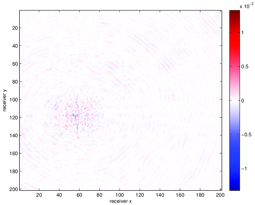
Results

We compare using HT tensor interpolation for the aforementioned data volume with NFT regularization and without regularization, the latter being equivalent to nearest neighbor binning on an interpolation problem with 75% randomly missing receivers. We run our optimization code for 15 iterations and display the results in Figure 3. Using this approach, we are able to successfully account for the off grid nature of our sampling and greatly improve upon our results when merely interpolating with binning.

Conclusion

In this work, we have introduced a low-rank tensor method for interpolating missing-trace seismic data sampled on an irregular grid. Our method is fast, SVD-free, and much more accurate than merely binning data before interpolation. Moreover, owing to the fast convergence of our baseline tensor completion algorithm, we have the flexibility of choosing different regularization operators that balance speed of application with accuracy of the signal model.