Preconditioned training of normalizing flows for variational inference in inverse problems

Ali Siahkoohi

Georgia Institute of Technology

Gabrio Rizzuti

Georgia Institute of Technology

Mathias Louboutin

Georgia Institute of Technology

Philipp A. Witte

Microsoft

Felix J. Herrmann

Georgia Institute of Technology

Introduction

Our aim is to perform approximate Bayesian inference for inverse problems characterized by computationally expensive forward operators, \(F: \mathcal{X} \rightarrow \mathcal{Y}\), with a data likelihood, \(\pi_{\text{like}} (\boldsymbol{y} \mid \boldsymbol{x})\): \[ \begin{equation} \boldsymbol{y} = F (\boldsymbol{x}) + \boldsymbol{\epsilon}, \label{fwd-op} \end{equation} \] where \(\boldsymbol{x} \in \mathcal{X}\) is the unknown model, \(\boldsymbol{y} \in \mathcal{Y}\) the observed data, and \(\boldsymbol{\epsilon} \sim \mathrm{N}(\boldsymbol{0}, \sigma^2 \boldsymbol{I})\) the measurement noise. Given a prior density, \(\pi_{\text{prior}}(\boldsymbol{x})\), variational inference (VI, Jordan et al., 1999) based on normalizing flows (NFs, Rezende and Mohamed, 2015) can be used where the Kullback-Leibler (KL) divergence is minimized between the predicted and the target—i.e., high-fidelity, posterior density \(\pi_{\text{post}} (\boldsymbol{x} \mid \boldsymbol{y} )\) (Liu and Wang, 2016; Kruse et al., 2019; Rizzuti et al., 2020; Siahkoohi et al., 2020; H. Sun and Bouman, 2020): \[ \begin{equation} \min_{\theta}\, \mathbb{E}\,_{\boldsymbol{z} \sim \pi_{z}(\boldsymbol{z})} \bigg [ \frac{1}{2\sigma^2} \left \| F \big(T_{\theta} (\boldsymbol{z}) \big) - \boldsymbol{y} \right \|_2^2 -\log \pi_{\text{prior}} \big (T_{\theta} (\boldsymbol{z}) \big ) -\log \Big | \det \nabla_{z} T_{\theta} (\boldsymbol{z}) \Big | \bigg ]. \label{hint2-obj} \end{equation} \] In the above expression, \(T_{\theta} : \mathcal{Z}_x \to \mathcal{X}\) denotes a NF with parameters \(\boldsymbol{\theta}\) and a Gaussian latent variable \(\boldsymbol{z} \in \mathcal{Z}_x\). The above objective consists of the data likelihood term, regularization on the output of the NF, and a log-determinant term that is related to the entropy of the NF output. The last term is necessarily to prevent the output of the NF from collapsing on the maximum a posteriori estimate. For details regarding the derivation of the objective in Equation (\(\ref{hint2-obj}\)), we refer to Appendix A. During training, we replace the expectation by Monte-Carlo averaging using mini-batches of \(\boldsymbol{z}\). After training, samples from the approximated posterior, \(\pi_{\theta}(\boldsymbol{x} \mid \boldsymbol{y}) \approx \pi_{\text{post}} (\boldsymbol{x} \mid \boldsymbol{y})\), can be drawn by evaluating \(T_{\theta}(\boldsymbol{z})\) for \(\boldsymbol{z} \sim \pi_{z}(\boldsymbol{z})\) (Kruse et al., 2019). It is important to note that Equation (\(\ref{hint2-obj}\)) trains a NF specific to the observed data \(\boldsymbol{y}\). While the above VI formulation in principle allows us to train a NF to generate samples from the posterior given a single observation \(\boldsymbol{y}\), this variational estimate requires access to a prior density, and the training calls for repeated evaluations of the forward operator, \(F\), as well as the adjoint of its Jacobian, \(\nabla {F}^\top\). As in multi-fidelity Markov chain Monte Carlo (MCMC) sampling (Peherstorfer and Marzouk, 2019), the costs associated with the forward operator may become prohibitive even though VI-based methods are known to have computational advantages over MCMC (Blei et al., 2017).

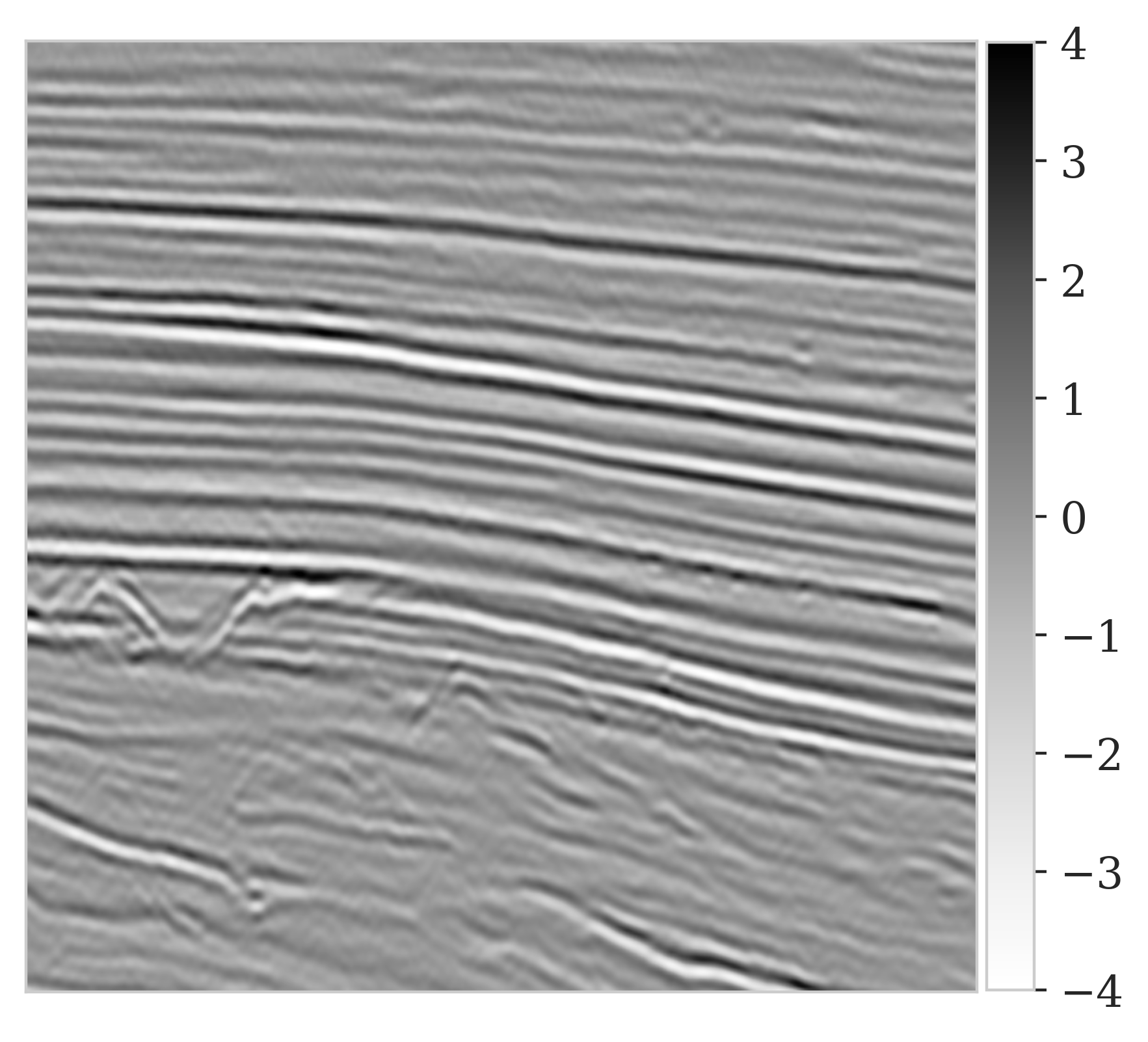
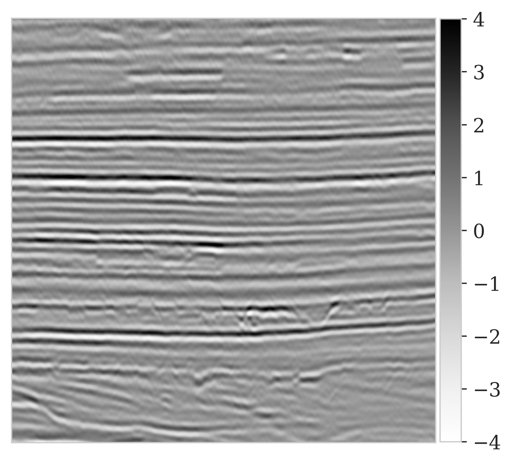
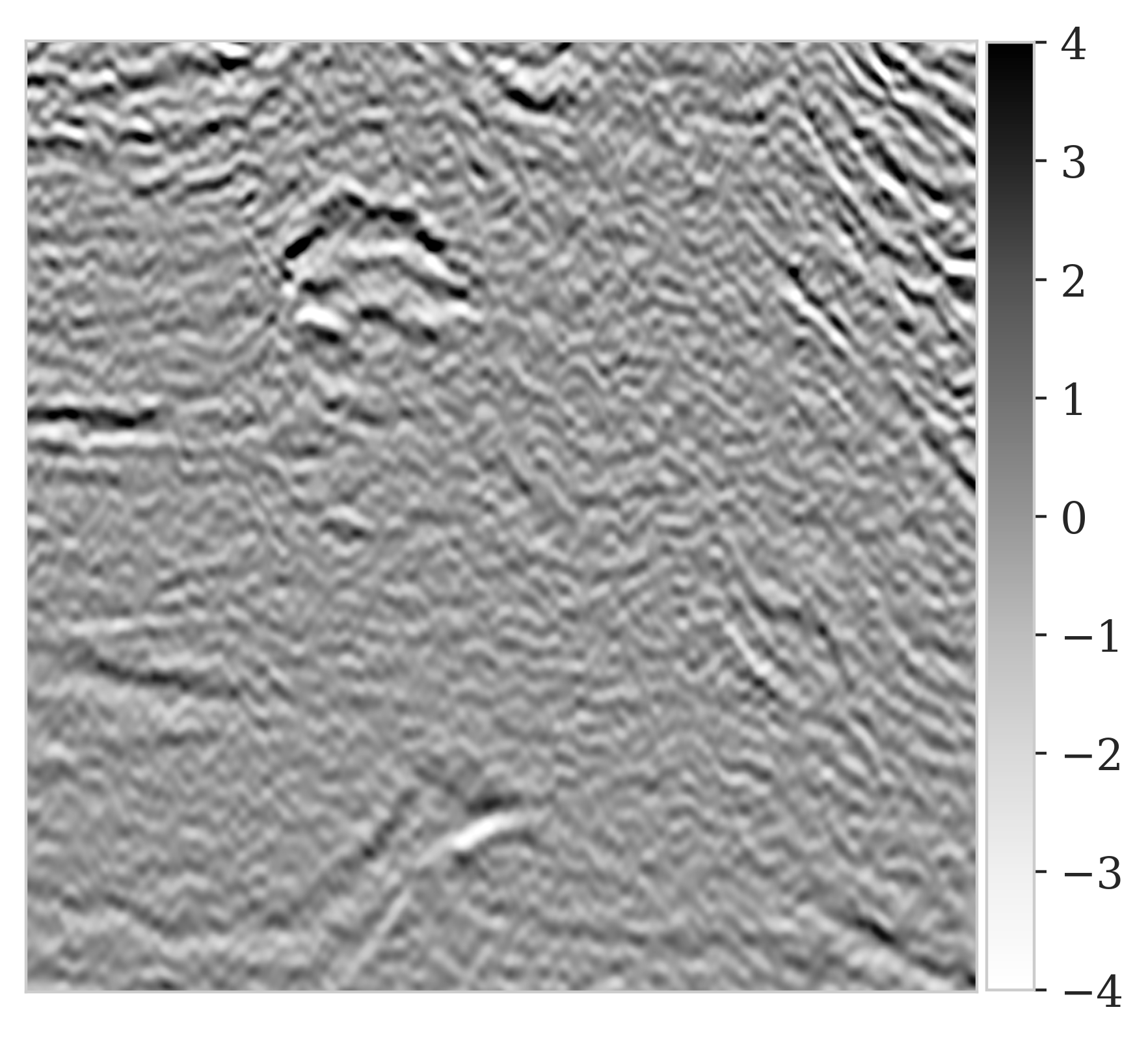
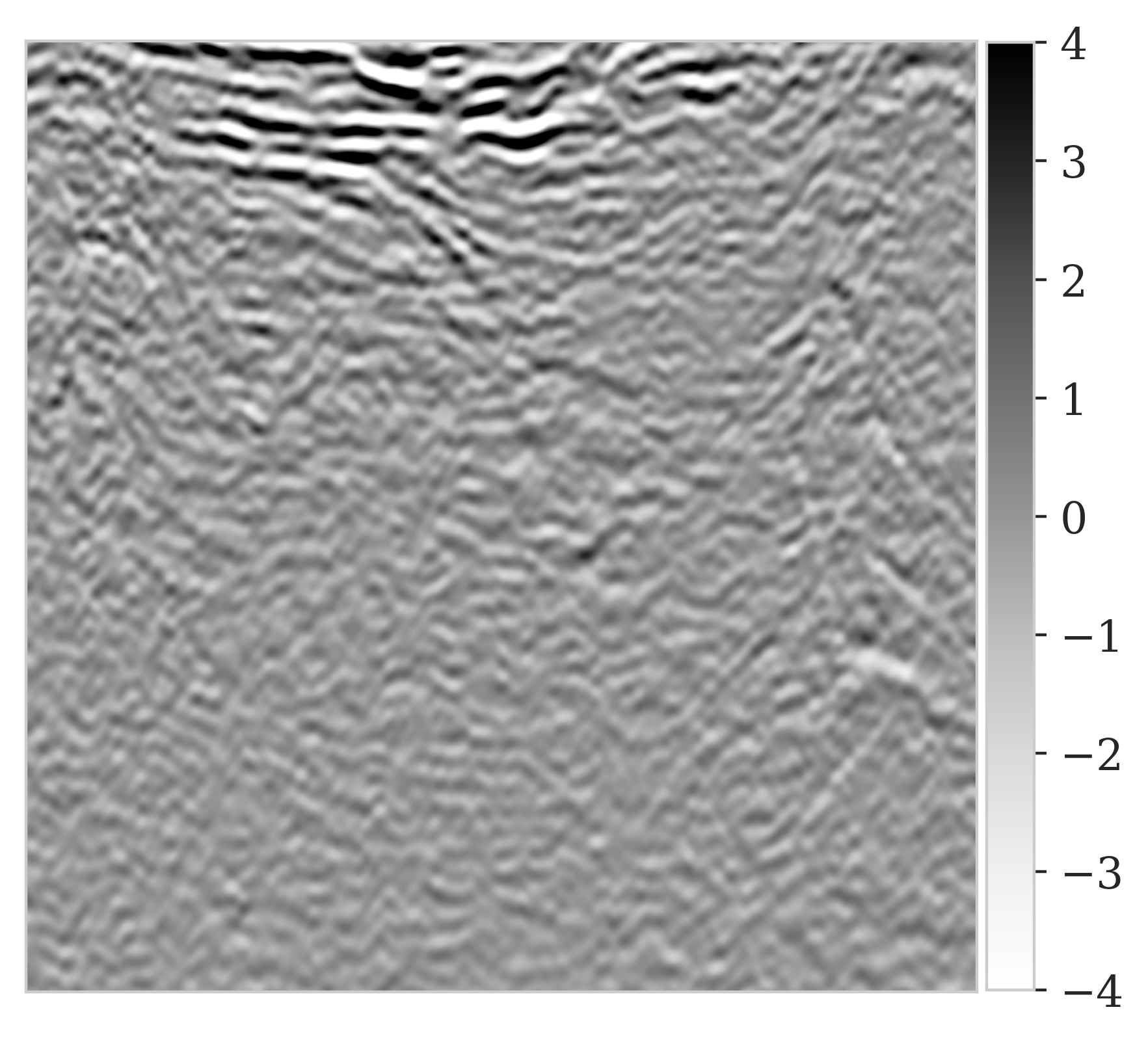
Aside from the above computational considerations, reliance on having access to a prior may be problematic especially when dealing with images of the Earth’s subsurface, which are the result of complex geological processes that do not lend themselves to be easily captured by hand-crafted priors. Under these circumstances, data-driven priors—or even better data-driven posteriors obtained by training over model and data pairs sampled from the joint distribution, \(\widehat{\pi}_{y, x} (\boldsymbol{y}, \boldsymbol{x})\)—are preferable. More specifically, we follow Kruse et al. (2019), Kovachki et al. (2020), and Baptista et al. (2020), and formulate the objective function in terms of a block-triangular conditional NF, \(G_{\phi} : \mathcal{Y} \times \mathcal{X} \to \mathcal{Z}_y \times \mathcal{Z}_x\), with latent space \(\mathcal{Z}_y \times \mathcal{Z}_x\): \[ \begin{equation} \begin{aligned} & \min_{\phi}\, \mathbb{E}\,_{\boldsymbol{y}, \boldsymbol{x} \sim \widehat{\pi}_{y, x} (\boldsymbol{y}, \boldsymbol{x})}\, \left [ \frac{1}{2} \left \| G_{\phi} (\boldsymbol{y}, \boldsymbol{x}) \right \|^2 - \log \Big|\det \nabla_{y, x}\, G_{\phi} (\boldsymbol{y}, \boldsymbol{x}) \Big | \right ], \\ & \text{where} \quad G_{\phi}(\boldsymbol{y}, \boldsymbol{x}) =\begin{bmatrix} G_{\phi_y} (\boldsymbol{y}) \\G_{\phi_x} (\boldsymbol{y}, \boldsymbol{x}) \end{bmatrix}, \ \boldsymbol{\phi} = \left \{ \boldsymbol{\phi}_y , \boldsymbol{\phi}_x \right \}. \end{aligned} \label{hint3-obj} \end{equation} \] Thanks to the block-triangular structure of \(G_{\phi}\), samples of the approximated posterior, \(\pi_{\phi}(\boldsymbol{x} \mid \boldsymbol{y}) \approx \pi_{\text{post}} (\boldsymbol{x} \mid \boldsymbol{y})\) can be drawn by evaluating \(G_{\phi_x}^{-1} (G_{\phi_y} (\boldsymbol{y}), \boldsymbol{z})\) for \(\boldsymbol{z} \sim \pi_{z}(\boldsymbol{z})\) (Marzouk et al., 2016). Unlike the objective in Equation (\(\ref{hint2-obj}\)), training \(G_{\phi}\) does not involve multiple evaluations of \(F\) and \(\nabla F^\top\), nor does it require specifying a prior density. However, its success during inference heavily relies on having access to training pairs from the joint distribution, \(\boldsymbol{y}, \boldsymbol{x}\sim \widehat{\pi}_{y, x} (\boldsymbol{y}, \boldsymbol{x})\). Unfortunately, unlike medical imaging, where data is abundant and variability among patients is relatively limited, samples from the joint distribution are unavailable in geophysical applications. Attempts have been made to address this lack of training pairs including the generation of simplified artificial geological models (Mosser et al., 2019), but these approaches cannot capture the true heterogeneity exhibited by the Earth’s subsurface. This is illustrated in Figure 1, which shows several true seismic image patches drawn from the Parihaka dataset. Even though samples are drawn from a single data set, they illustrate significant differences between shallow (Figures 1a and 1b) and deeper (Figures 1c and 1d) sections.

To meet the challenges of computational cost, heterogeneity and lack of access to training pairs, we propose a preconditioning scheme where the two described VI methods are combined to:

1. take maximum advantage of available samples from the joint distribution \(\widehat{\pi}_{y, x} (\boldsymbol{y}, \boldsymbol{x})\), to pretrain \(G_{\phi}\) by minimizing Equation (\(\ref{hint3-obj}\)). We only incur these costs once, by training this NF beforehand. As these samples typically come from a different (neighboring) region, they are considered as low-fidelity;

2. exploit the invertibility of \(G_{\phi_x} (\boldsymbol{y}, \,\cdot\,)\), which gives us access to a low-fidelity posterior density, \(\pi_{\phi}(\boldsymbol{x} \mid \boldsymbol{y})\). For a given \(\boldsymbol{y}\), this trained (conditional) prior can be used in Equation (\(\ref{hint2-obj}\));

3. initialize \(T_{\theta}\) with weights from the pretrained \(G_{\phi_x}^{-1}\). This initialization can be considered as an instance of transfer learning (Yosinski et al., 2014), and we expect a considerable speed-up when solving Equation \(\eqref{hint2-obj}\). This is important since it involves inverting \(F\), which is computationally expensive.

Related work

In the context of variational inference for inverse problems with expensive forward operators, Herrmann et al. (2019) train a generative model to sample from the posterior distribution, given indirect measurements of the unknown model. This approach is based on an Expectation Maximization technique, which infers the latent representation directly instead of using an inference encoding model. While that approach allows for inclusion of hand-crafted priors, capturing the posterior is not fully developed. Like Kovachki et al. (2020), we also use a block-triangular map between the joint model and data distribution and their respective latent spaces to train a network to generate samples from the conditional posterior. By imposing an additional monotonicity constraint, these authors train a generative adversarial network (GAN, Goodfellow et al., 2014) to directly sample from the posterior distribution. To allow for scalability to large scale problems, we work with NFs instead, because they allow for more memory efficient training (Leemput et al., 2019; Putzky and Welling, 2019; Peters et al., 2020; Peters and Haber, 2020). Our contribution essentially corresponds to a reformulation of M. D. Parno and Marzouk (2018) and Peherstorfer and Marzouk (2019). In that work, transport-based maps are used as non-Gaussian proposal distributions during MCMC sampling. As part of the MCMC, this transport map is then tuned to match the target density, which improves the efficiency of the sampling. Peherstorfer and Marzouk (2019) extend this approach by proposing a preconditioned MCMC sampling technique where a transport-map trained to sample from a low-fidelity posterior distribution is used as a preconditioner. This idea of multi-fidelity preconditioned MCMC inspired our work where we setup a VI objective instead. We argue that this formulation can be faster and may be easier to scale to large-scale Bayesian inference problems (Blei et al., 2017).

Finally, there is a conceptional connection between our work and previous contributions on amortized variational inference (Gershman and Goodman, 2014), including an iterative refinement step (Hjelm et al., 2016; Krishnan et al., 2018; Kim et al., 2018; Marino et al., 2018). Although similar in spirit, our approach is different from these attempts because we adapt the weights of our conditional generative model to account for the inference errors instead of correcting the inaccurate latent representation of the out-of-distribution data.

Multi-fidelity preconditioning scheme

For an observation \(\boldsymbol{y}\), we define a NF \(T_{\phi_x} : \mathcal{Z}_x \to \mathcal{X}\) as \[ \begin{equation} T_{\phi_x}(\boldsymbol{z}):= G_{\phi_x}^{-1} (G_{\phi_y} (\boldsymbol{y}), \boldsymbol{z}), \label{low-fidelity-NF} \end{equation} \] where we obtain \(\boldsymbol{\phi} = \left \{ \boldsymbol{\phi}_y , \boldsymbol{\phi}_x \right \}\) by training \(G_{\phi}\) through minimizing the objective function in Equation (\(\ref{hint3-obj}\)). To train \(G_{\phi}\), we use available low-fidelity training pairs \(\boldsymbol{y}, \boldsymbol{x} \sim \widehat{\pi}_{y, x} (\boldsymbol{y}, \boldsymbol{x})\). We perform this training phase beforehand, similar to the pretraining phase during transfer learning (Yosinski et al., 2014). Thanks to the invertibility of \(G_{\phi}\), it provides an expression for the posterior. We refer to this posterior as low-fidelity because the network is trained with often scarce and out-of-distribution training pairs. Because the Earth’s heterogeneity does not lend itself to be easily captured by hand-crafted priors, we argue that this NF can still serve as a (conditional) prior in Equation (\(\ref{hint2-obj}\)): \[ \begin{equation} \pi_{\text{prior}} (\boldsymbol{x}) := \pi_{\boldsymbol{z}} \big(G_{\phi_x} (\boldsymbol{y}, \boldsymbol{x}) \big )\, \Big | \det \nabla_{x} G_{\phi_x} (\boldsymbol{y}, \boldsymbol{x}) \Big |. \label{low-fidelity-post} \end{equation} \] To train the high-fidelity NF given observed data \(\boldsymbol{y}\), we minimize the KL divergence between the predicted and the high-fidelity posterior density, \(\pi_{\text{post}} (\boldsymbol{x} \mid \boldsymbol{y} )\) (Liu and Wang, 2016; Kruse et al., 2019) \[ \begin{equation} \min_{\phi_x}\, \mathbb{E}_{\boldsymbol{z} \sim \pi_{z}(\boldsymbol{z})} \bigg [ \frac{1}{2\sigma^2} \left \| F \big(T_{\phi_x} (\boldsymbol{z}) \big) - \boldsymbol{y} \right \|_2^2 -\log \pi_{\text{prior}} \big (T_{\phi_x} (\boldsymbol{z}) \big ) -\log \Big | \det \nabla_{z} T_{\phi_x} (\boldsymbol{z}) \Big | \bigg ], \label{hint2-obj-finetune} \end{equation} \] where the prior density of Equation (\(\ref{low-fidelity-post}\)) is used. Notice that this minimization problem differs from the one stated in Equation (\(\ref{hint2-obj}\)). Here, the optimization involves “fine-tuning” the low-fidelity network parameters \(\phi_x\) introduced in Equation (\(\ref{hint3-obj}\)). Moreover, this low-fidelity network is also used as a prior. While other choices exist for the latter—e.g., it could be replaced or combined with a hand-crafted prior in the form of constraints (Peters et al., 2019) or by a separately trained data-driven prior (Mosser et al., 2019), using the low-fidelity posterior as a prior (cf. Equation (\(\ref{low-fidelity-post}\))) has certain distinct advantages. First, it removes the need for training a separate data-driven prior model. Second, use of the low-fidelity posterior may be more informative (Yang and Soatto, 2018) than its unconditional counterpart because it is conditioned by the observed data \(\boldsymbol{y}\). In addition, our multi-fidelity approach has strong connections with online variational Bayes (Zeno et al., 2018) where data arrives sequentially and previous posterior approximates are used as priors for subsequent approximations.

In summary, the problem in Equation \(\eqref{hint2-obj-finetune}\) can be interpreted as an instance of transfer learning (Yosinski et al., 2014) for conditional NFs. This formulation is particularly useful for inverse problems with expensive forward operators, where access to high fidelity training samples, i.e. samples from the target distribution, is limited. In the next section, we present two numerical experiments designed to show the speed-up and accuracy gained with our proposed multi-fidelity formulation.

Numerical experiments

We present two synthetic examples aimed at verifying the anticipated speed-up and increase in accuracy of the predicted posterior density via our multi-fidelity preconditioning scheme. The first example is a two-dimensional problem where the posterior density can be accurately and cheaply sampled via MCMC. The second example demonstrates the effect of the preconditioning scheme in a seismic compressed sensing (Candes et al., 2006; Donoho, 2006) problem. Details regarding training hyperparameters and the NF architectures are included in Appendix B. Code to reproduce our results are made available on GitHub. Our implementation relies on InvertibleNetworks.jl (P. Witte et al., 2020), a recently-developed memory-efficient framework for training invertible networks in the Julia programming language.

2D toy example

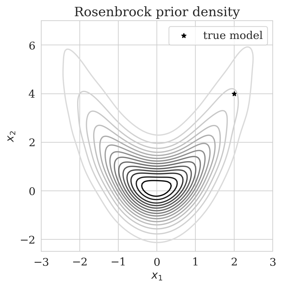
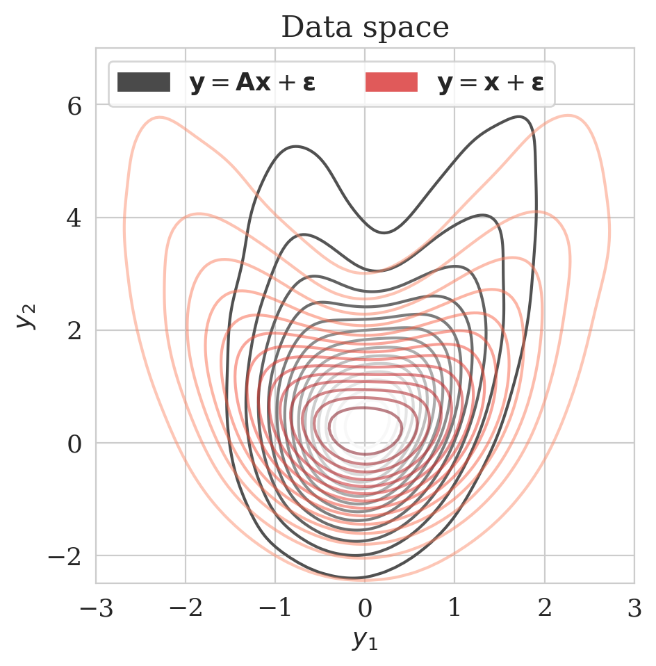
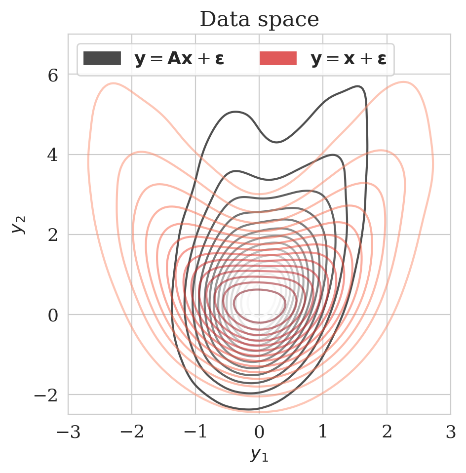
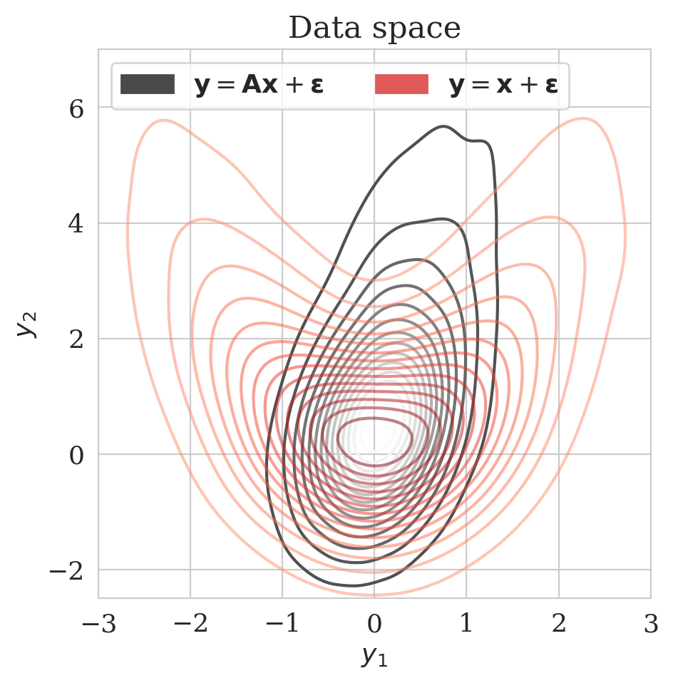
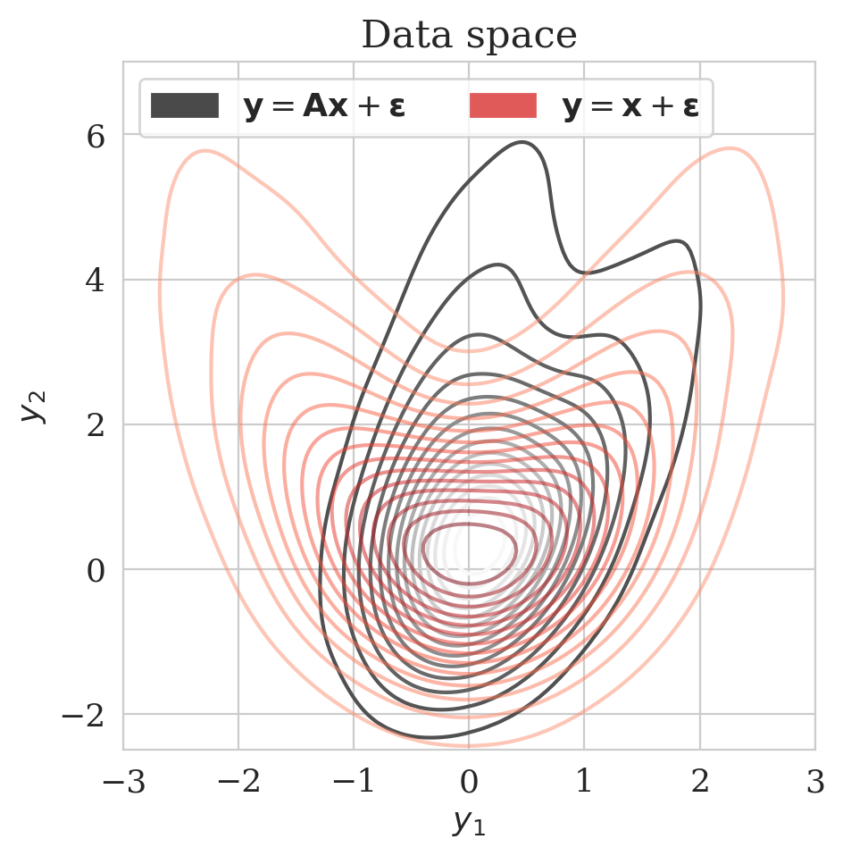
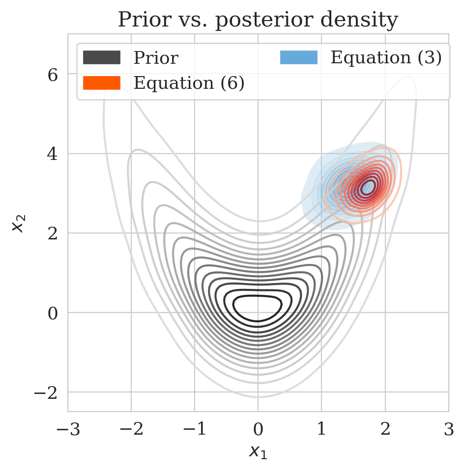
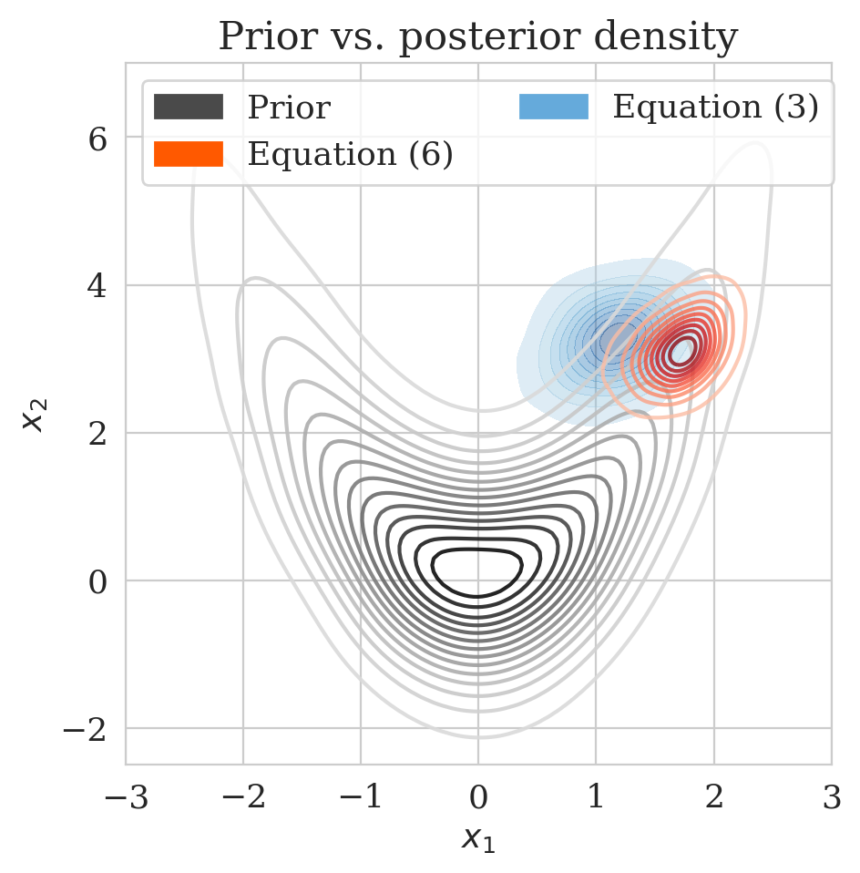
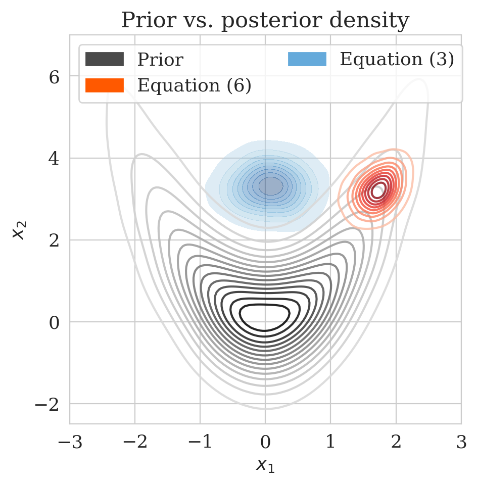
To illustrate, the advantages of working with our multi-fidelity scheme, we consider the 2D Rosenbrock distribution, \(\pi_{\text{prior}} (\boldsymbol{x}) \propto \exp \left( - \frac{1}{2} x_{1}^{2} - \left(x_{2}-x_{1}^{2} \right)^{2}\right)\), plotted in Figure 2a. High-fidelity data \(\boldsymbol{y} \in\mathbb{R}^{2}\) are generated via \(\boldsymbol{y} = \boldsymbol{A}\, \boldsymbol{x} + \boldsymbol{\epsilon}\), where \(\boldsymbol{\epsilon} \sim \mathrm{N}(\boldsymbol{0}, 0.4^2 \boldsymbol{I})\) and \(\boldsymbol{A} \in \mathbb{R}^{2 \times 2}\) is a forward operator. To control the discrepancy between the low- and high-fidelity samples, we set \(\boldsymbol{A}\) equal to \(\bar{\boldsymbol{A}} \mathbin{/} \rho (\bar{\boldsymbol{A}})\), where \(\rho ( \cdot)\) is the spectral radius of \(\bar{\boldsymbol{A}} = \boldsymbol{\Gamma} + \gamma \boldsymbol{I}\), \(\boldsymbol{\Gamma} \in \mathbb{R}^{2 \times 2}\) has independent and normally distributed entries, and \(\gamma = 3\). By choosing smaller values for \(\gamma\), we make \(\boldsymbol{A}\) more dissimilar to the identity matrix, therefore increasing the discrepancy between the low- and high-fidelity posterior.

Figure 2b depicts the low- (purple) and high-fidelity (red) data densities. The dark star represents the unknown model. Low-fidelity data samples are generated with the identity as the forward operator. During the pretraining phase conducted beforehand, we minimize the objective function in Equation (\(\ref{hint3-obj}\)) for \(25\) epochs.

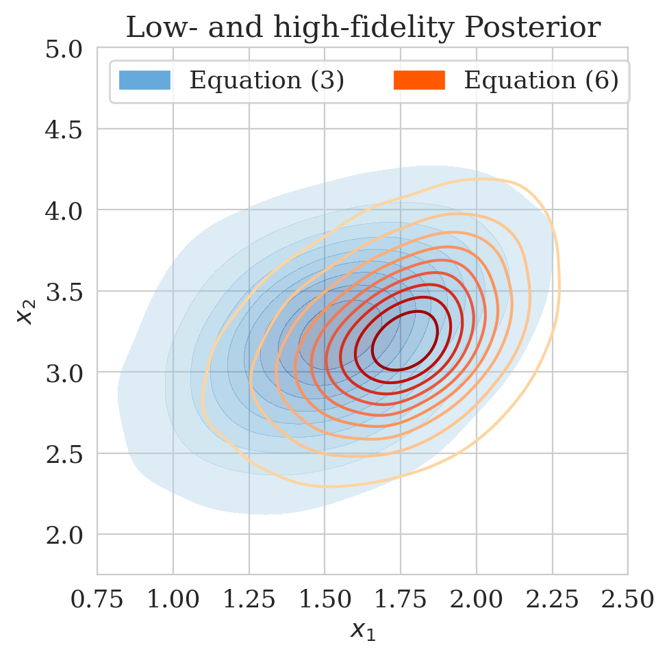
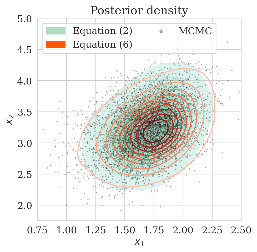
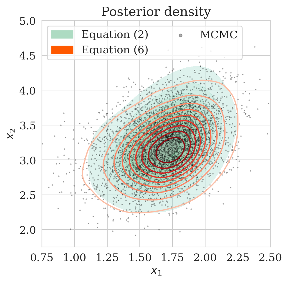
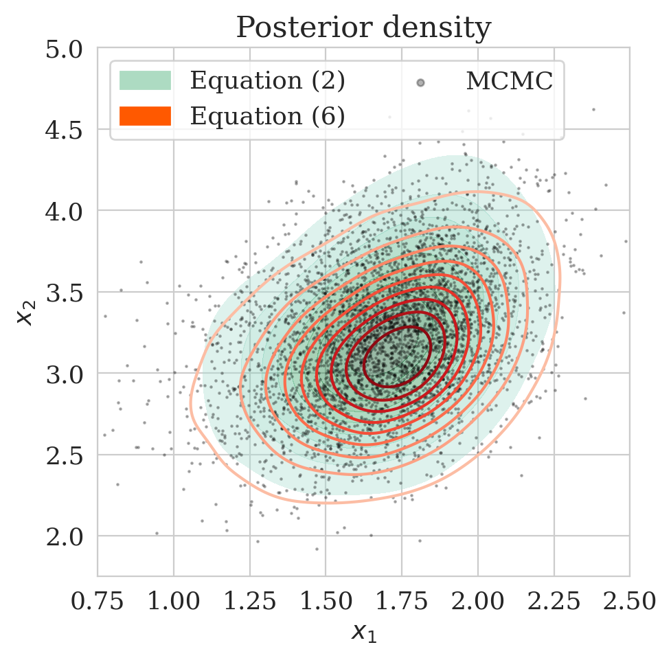
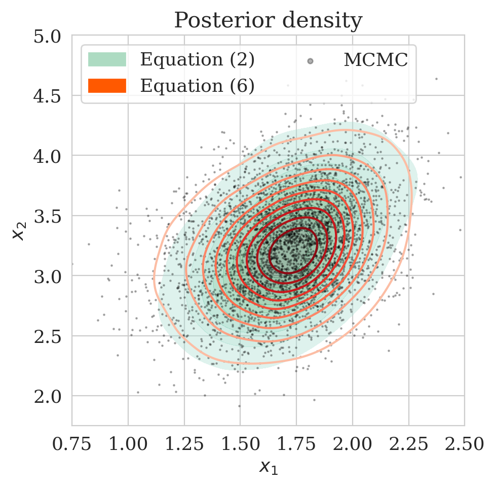
The pretrained low-fidelity posterior is subsequently used to precondition the minimization of (\(\ref{hint2-obj-finetune}\)) given observed data \(\boldsymbol{y}\). The resulting low- and high-fidelity estimates for the posterior as plotted in Figure 2c differ significantly. In Figure (2d), the accuracy of the proposed method is verified by comparing the approximated high-fidelity posterior density (orange contours) with the approximation (in green) obtained by minimizing the objective of Equation \(\eqref{hint2-obj}\). The overlap between the orange contours and the green shaded area confirms consistency between the two methods. To assess the accuracy of the estimated densities themselves, we also include samples from the posterior (dark circles) obtained via stochastic gradient Langevin dynamics (Welling and Teh, 2011), an MCMC sampling technique. As expected, the estimated posterior densities with and without the preconditioning scheme are in agreement with the MCMC samples.

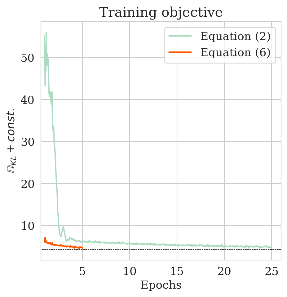
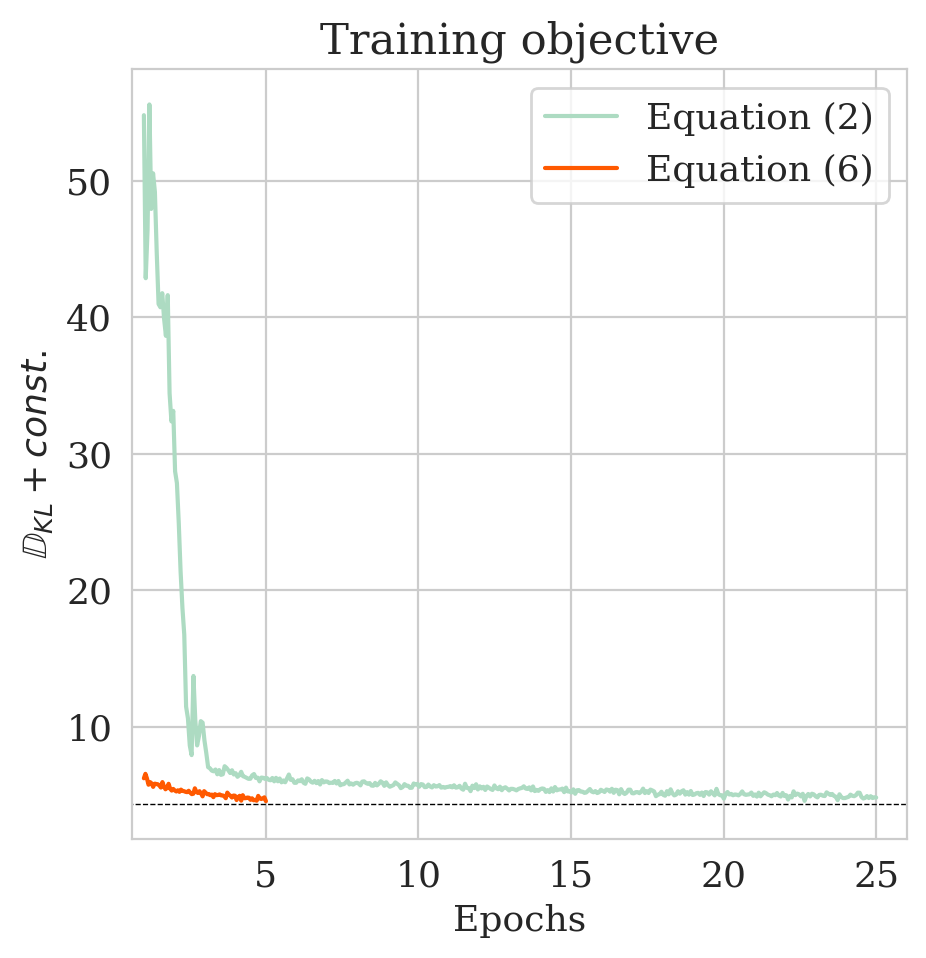
Finally, to illustrate the performance our multi-fidelity scheme, we consider the convergence plot in Figure 2e where the objective values of Equations (\(\ref{hint2-obj}\)) and (\(\ref{hint2-obj-finetune}\)) are compared. As explained in Appendix A, the values of the objective functions correspond to the KL divergence (plus a constant) between the posterior given by Equation (\(\ref{hint2-obj}\)) and the posterior distribution obtained by our multi-fidelity approach (Equation (\(\ref{hint2-obj-finetune}\))). As expected, the multi-fidelity objective converges much faster because of the “warm start”. In addition, the updates of \(T_{\phi_x}\) via Equation (\(\ref{hint2-obj-finetune}\)) succeed in bringing down the KL divergence within only five epochs (see orange curve), whereas it takes \(25\) epochs via the objective in Equation \(\eqref{hint2-obj}\) to reach approximately the same KL divergence. This pattern holds for smaller values of \(\gamma\) too as indicated in Table 1. According to Table 1, the improvements by our multi-fidelity method become more pronounced if we decrease the \(\gamma\). This behavior is to be expected since the samples used for pretraining are more and more out of distribution in that case. We refer to Appendix C for additional figures for different values of \(\gamma\).

\(\gamma\)	Low-fidelity	Without preconditioning	With preconditioning
\(3\)	\(6.13\)	\(4.88\)	\(4.66\)
\(2\)	\(8.43\)	\(5.60\)	\(5.26\)
\(1\)	\(8.84\)	\(6.26\)	\(6.51\)
\(0\)	\(14.73\)	\(8.41\)	\(8.45\)

Seismic compressed sensing example

This experiment is designed to show challenges with geophysical inverse problems due to the Earth’s strong heterogeneity. We consider the inversion of noisy indirect measurements of image patches \(\boldsymbol{x} \in \mathbb{R}^{256 \times 256}\) sampled from deeper parts of the Parihaka seismic dataset. The observed measurements are given by \(\boldsymbol{y} = \boldsymbol{A} \boldsymbol{x} + \boldsymbol{\epsilon}\) where \(\boldsymbol{\epsilon} \sim \mathrm{N}(\boldsymbol{0}, 0.2^2 \boldsymbol{I})\). For simplicity, we chose \(\boldsymbol{A} = {\boldsymbol{M}}^T {\boldsymbol{M}}\) with \({\boldsymbol{M}}\) a compressing sensing matrix with \(66.66\,\)% subsampling. The measurement vector \(\boldsymbol{y}\) corresponds to a pseudo-recovered model contaminated with noise.

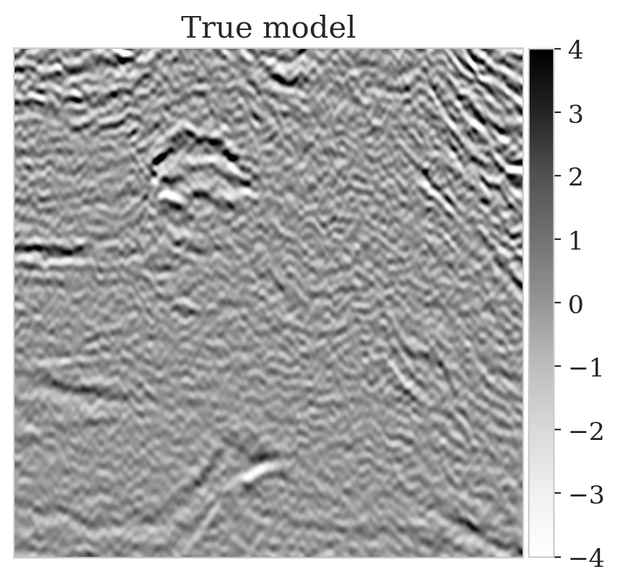
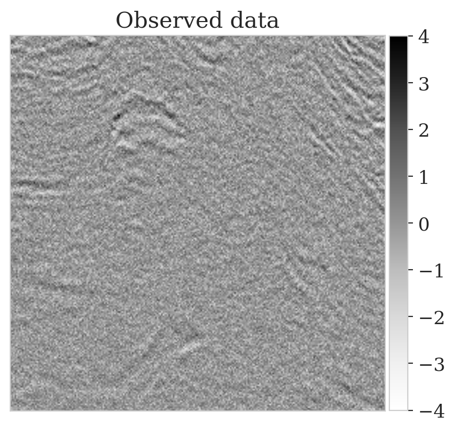
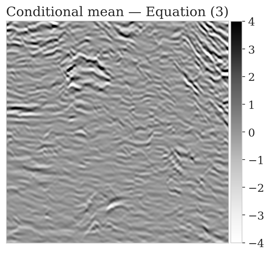
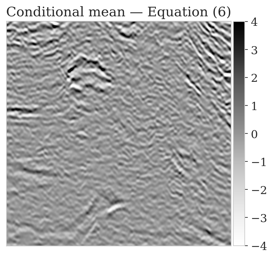
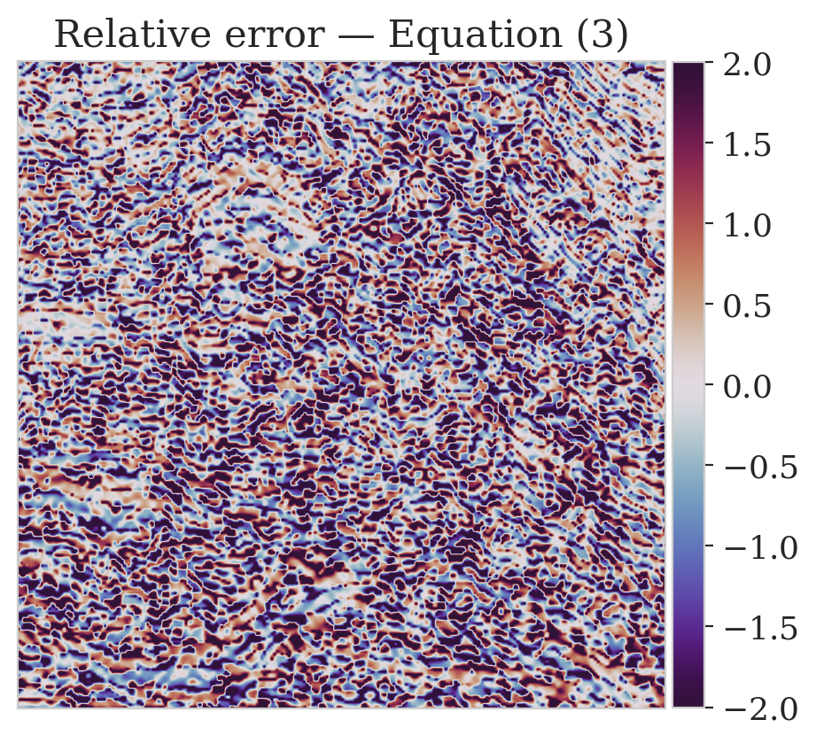
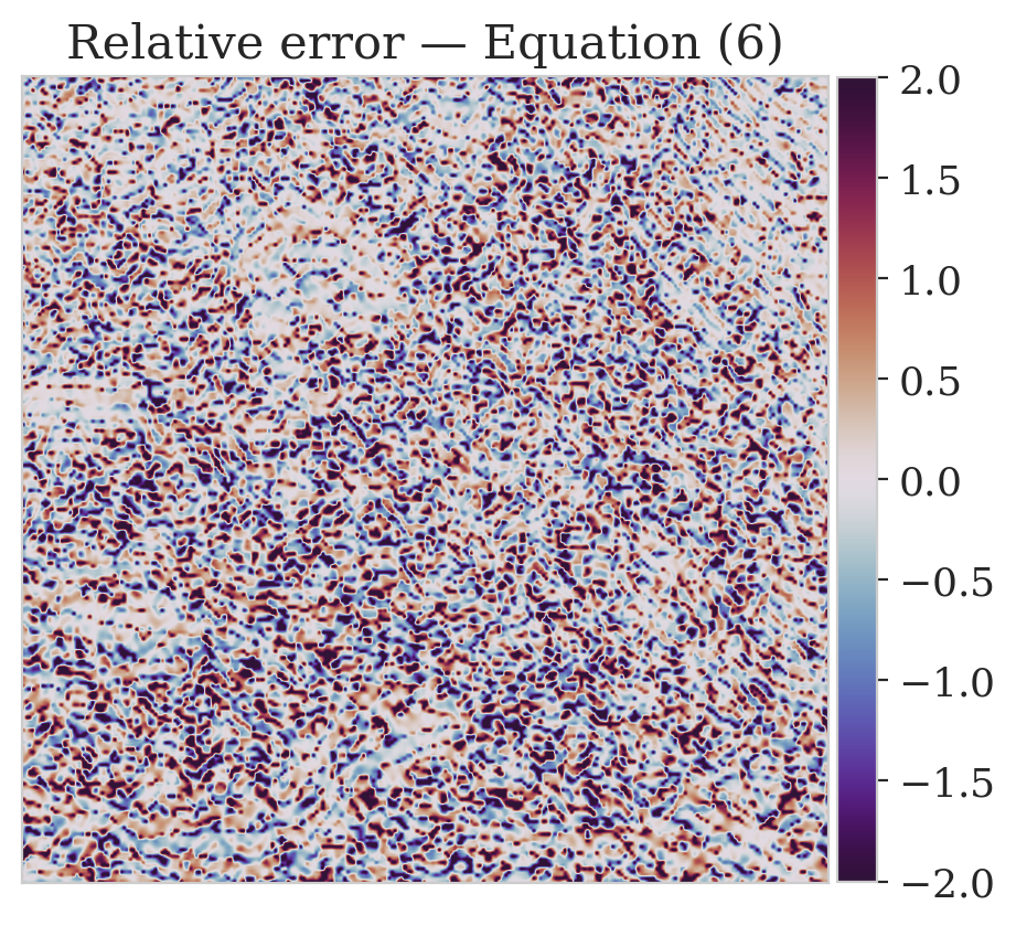
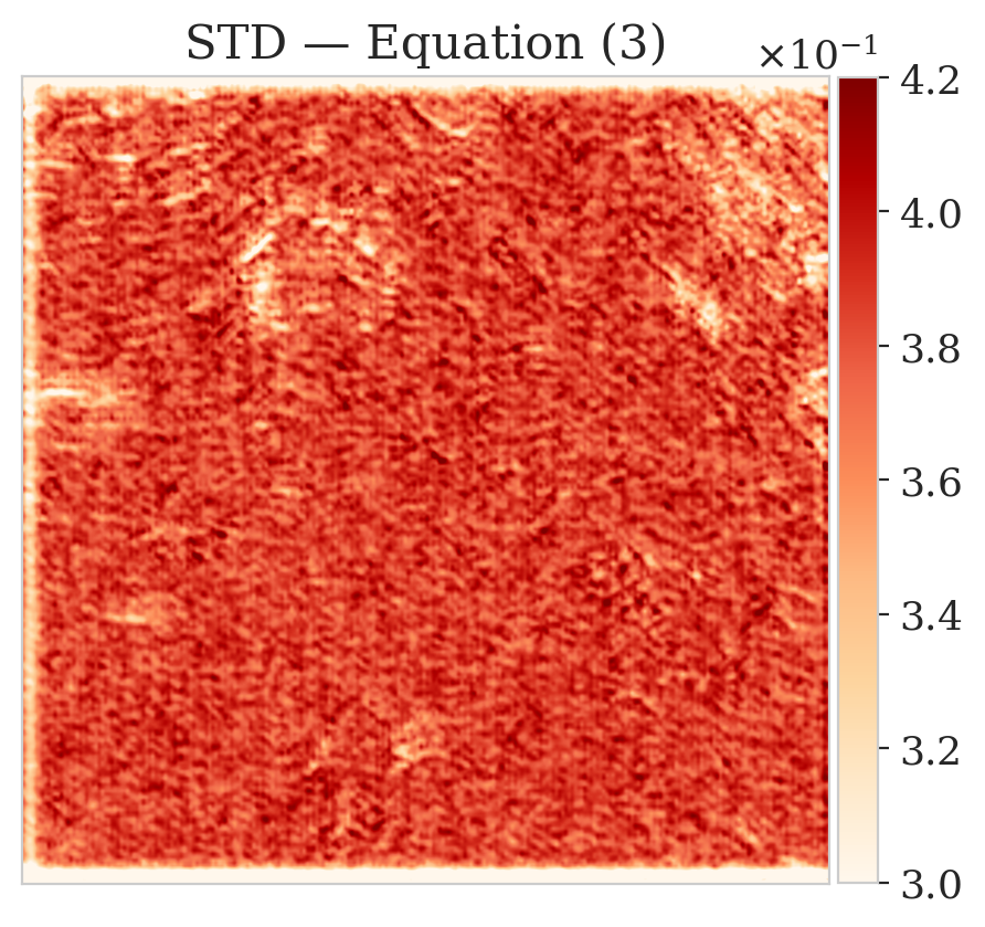
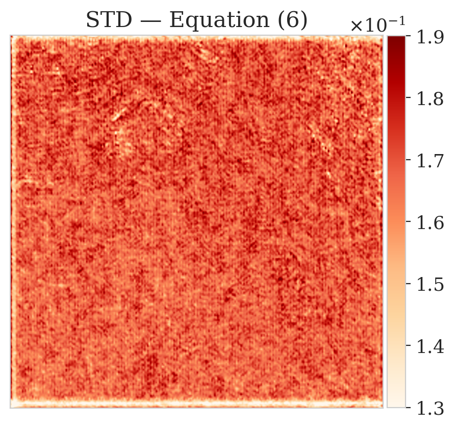
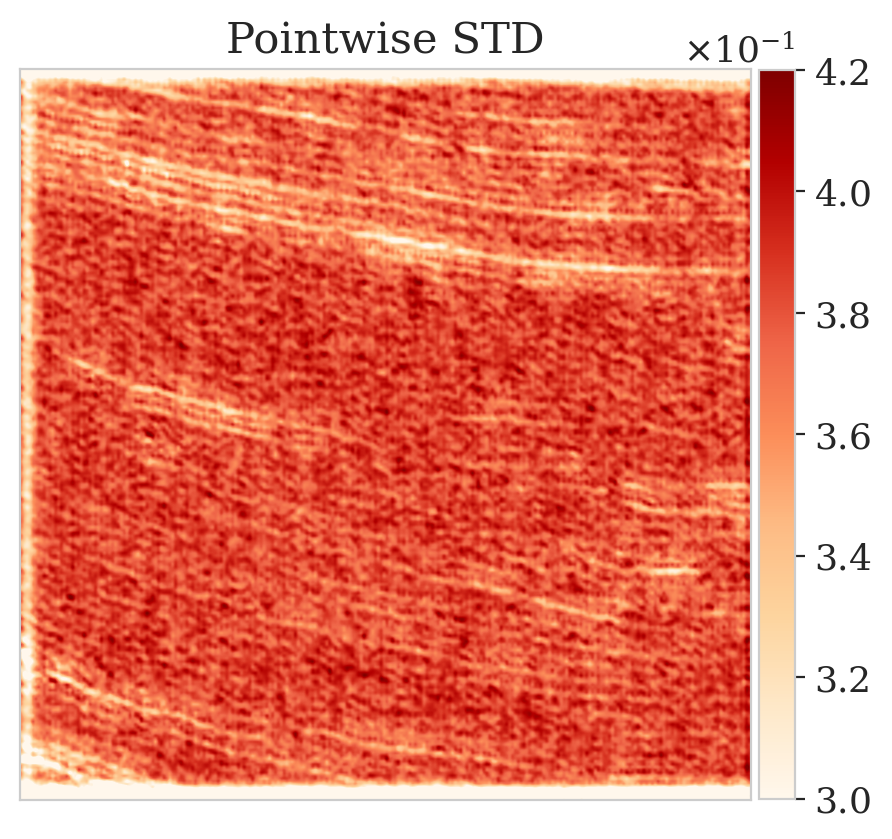
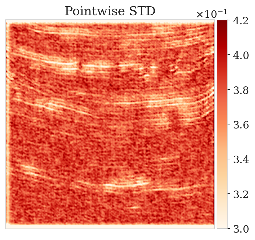
To mimic a realistic situation in practice, we change the likelihood distribution by reducing the standard deviation of the noise to \(0.01\) in combination with using image patches sampled from the shallow part of the Parihaka dataset. As we have seen in Figure 1, these patches differ in texture. Given pairs \(\boldsymbol{y}, \boldsymbol{x} \sim \widehat{\pi}_{y, x} (\boldsymbol{y}, \boldsymbol{x})\), we pretrain our network by minimizing Equation (\(\ref{hint3-obj}\)). Figures 3a and 3b contain a pair not used during pretraining. Estimates for the conditional mean and standard deviation obtained by drawing \(1000\) samples from the pretrained conditional NF for the noisy indirect measurement (Figure 3b) are included in Figures 3c and 3d. Both estimates exhibit the expected behavior because the examples in Figure 3a and 3b are within the distribution. As anticipated, this observation no longer holds if we apply this pretrained network to indirect data depicted in Figure 3f, which is sampled from the deeper part. However, these results are significantly improved when the pretrained network is fine-tuned by minimizing Equation (\(\ref{hint2-obj-finetune}\)). After fine tuning, the fine details in the image are recovered (compare Figures 3g and 3h). This improvement is confirmed by the relative errors plotted in Figures 3i and 3j, as well as by the reduced standard deviation (compare Figures 3k and 3l).

Conclusions

Inverse problems in fields such as seismology are challenging for several reasons. The forward operators are complex and expensive to evaluate numerically while the Earth is highly heterogeneous. To handle this situation and to quantify uncertainty, we propose a preconditioned scheme for training normalizing flows for Bayesian inference. The proposed scheme is designed to take full advantage of having access to training pairs drawn from a joint distribution, which for the reasons stated above is close but not equal to the actual joint distribution. We use these samples to train a normalizing flow via likelihood maximization leveraging the normalizing property. We use this pretrained low-fidelity estimate for the posterior as a prior and preconditioner for the actual variational inference on the observed data, which minimizes the Kullback-Leibler divergence between the predicted and the desired posterior density. By means of a series of examples, we demonstrate that our preconditioned scheme leads to considerable speed-ups compared to training a normalizing flow from scratch.

Mathematical derivations

Let \(f : \mathcal{Z} \to \mathcal{X}\) be a bijective transformation that maps a random variable \(\boldsymbol{z} \sim \pi_{z} (\boldsymbol{z})\) to \(\boldsymbol{x} \sim \pi_{x} (\boldsymbol{x})\). We can write the change of variable formula (Villani, 2009) that relates probability density functions \(\pi_{z}\) and \(\pi_{x}\) in the following manner: \[ \begin{equation} \pi_x (\boldsymbol{x}) = \pi_z (\boldsymbol{z})\, \Big | \det \nabla_{x} f^{-1} (\boldsymbol{x}) \Big |, \quad f (\boldsymbol{z}) = \boldsymbol{x}, \quad \boldsymbol{x} \in \mathcal{X}. \label{change-of-variable} \end{equation} \] This relation serves as the basis for the objective functions used throughout this paper.

Derivation of Equation (\(\ref{hint2-obj}\))

In Equation \(\ref{hint2-obj}\), we train a bijective transformation, denoted by \(T_{\theta} : \mathcal{Z}_x \to \mathcal{X}\), that maps the latent distribution \(\pi_{z_x}(\boldsymbol{z}_x)\) to the high-fidelity posterior density \(\pi_{\text{post}} (\boldsymbol{x} \mid \boldsymbol{y} )\). We optimize the parameters of \(T_{\theta}\) by minimizing the KL divergence between the push-forward density (Bogachev, V.I., 2006), denoted by \(\pi_{\theta} (\, \cdot \mid \boldsymbol{y}) := T_{\sharp}\, \pi_{z_x}\), and the posterior density: \[ \begin{equation} \begin{aligned} & \mathop{\rm arg\,min}_{\theta}\, \mathbb{D}_{\text{KL}} \left (\pi_{\theta} (\, \cdot \mid \boldsymbol{y}) \mid\mid \pi_{\text{post}} (\, \cdot \mid \boldsymbol{y}) \right ) \\ = & \mathop{\rm arg\,min}_{\theta}\, \mathbb{E}_{\boldsymbol{x} \sim \pi_{\theta} (\boldsymbol{x} \mid \boldsymbol{y})} \Big [ - \log \pi_{\text{post}} (\boldsymbol{x} \mid \boldsymbol{y} ) + \log \pi_{\theta} (\boldsymbol{x} \mid \boldsymbol{y}) \Big ]. \end{aligned} \label{hint2-obj-derivation} \end{equation} \] In the above expression, we can rewrite the expectation with respect to \(\pi_{\theta} (\boldsymbol{x} \mid \boldsymbol{y})\) as the expectation with respect to the latent distribution, followed by a mapping via \(T_{\theta}\)—i.e., \[ \begin{equation} \mathop{\rm arg\,min}_{\theta}\, \mathbb{E}_{\boldsymbol{z}_x \sim \pi_{z_x} (\boldsymbol{z})} \Big [ - \log \pi_{\text{post}} (T_{\theta} (\boldsymbol{z}_x) \mid \boldsymbol{y} ) + \log \pi_{\theta} (T_{\theta} (\boldsymbol{z}_x) \mid \boldsymbol{y}) \Big ]. \label{change-expectation} \end{equation} \] The last term in the expectation above can be further simplified via the change of variable formula in Equation (\(\ref{change-of-variable}\)). If \(\boldsymbol{x} = T_{\theta} (\boldsymbol{z}_x)\), then: \[ \begin{equation} \pi_{\theta} (\boldsymbol{x} \mid \boldsymbol{y}) = \pi_{z_x} (\boldsymbol{z}_x)\, \Big | \det \nabla_{x} T_{\theta} ^{-1} (\boldsymbol{x}) \Big | = \pi_{z_x} (\boldsymbol{z}_x)\, \Big | \det \nabla_{z_x} T_{\theta} (\boldsymbol{z}_x) \Big |^{-1}. \label{change-of-variable-hint2} \end{equation} \] The last equality in Equation (\(\ref{change-of-variable-hint2}\)) holds due to the invertibility of \(T_{\theta}\) and the differentiability of its inverse (inverse function theorem). By combining Equations (\(\ref{change-expectation}\)) and (\(\ref{change-of-variable-hint2}\)), we arrive at the following objective function for training \(T_{\theta}\):

\[ \begin{equation} \mathop{\rm arg\,min}_{\theta}\, \mathbb{E}_{\boldsymbol{z}_x \sim \pi_{z_x} (\boldsymbol{z})} \Big [ - \log \pi_{\text{post}} (T_{\theta} (\boldsymbol{z}_x) \mid \boldsymbol{y} ) + \log \pi_{z_x} (\boldsymbol{z}_x) -\log \Big | \det \nabla_{z_x} T_{\theta} (\boldsymbol{z}_x) \Big | \Big ]. \label{final-equ-hint2} \end{equation} \]

Finally, by ignoring the \(\log \pi_{z_x} (\boldsymbol{z}_x)\) term, which is constant with respect to \(\boldsymbol{\theta}\), using Bayes’ rule, and inserting our data likelihood model from Equation (\(\ref{fwd-op}\)), we derive Equation (\(\ref{hint2-obj}\)):

\[ \begin{equation} \min_{\theta}\, \mathbb{E}\,_{\boldsymbol{z}_x \sim \pi_{z_x}(\boldsymbol{z}_x)} \bigg [ \frac{1}{2\sigma^2} \left \| F \big(T_{\theta} (\boldsymbol{z}_x) \big) - \boldsymbol{y} \right \|_2^2 -\log \pi_{\text{prior}} \big (T_{\theta} (\boldsymbol{z}_x) \big ) -\log \Big | \det \nabla_{z_x} T_{\theta} (\boldsymbol{z}_x) \Big | \bigg ]. \label{hint2-obj-derived} \end{equation} \]

Next, based on this equation, we derive the objective function used in the pretraining phase.

Derivation of Equation (\(\ref{hint3-obj}\))

The derivation of objective in Equation (\(\ref{hint3-obj}\)) follows directly from the change of variable formula in Equation \(\ref{change-of-variable}\), applied to a bijective map, \(G^{-1}_{\phi} : \mathcal{Z}_y \times \mathcal{Z}_x \to \mathcal{Y} \times \mathcal{X}\), where \(\mathcal{Z}_y\) and \(\mathcal{Z}_y\) are Gaussian latent spaces. That is to say: \[ \begin{equation} \begin{split} \widehat{\pi}_{y, x} (\boldsymbol{y}, \boldsymbol{x}) = \pi_{z_y, z_x} (\boldsymbol{z}_y, \boldsymbol{z}_x)\, \Big | \det \nabla_{y, x} G_{\phi} (\boldsymbol{y}, \boldsymbol{x}) \Big |, \quad G_{\phi}(\boldsymbol{y}, \boldsymbol{x}) =\begin{bmatrix} \boldsymbol{z}_y \\\boldsymbol{z}_x \end{bmatrix}. \end{split} \label{change-of-variable-hint3} \end{equation} \] Given (low-fidelity) training pairs, \(\boldsymbol{y}, \boldsymbol{x} \sim \widehat{\pi}_{y, x} (\boldsymbol{y}, \boldsymbol{x})\), the maximum likelihood estimate of \(\boldsymbol{\phi}\) is obtained via the following objective: \[ \begin{equation} \begin{aligned} & \mathop{\rm arg\,max}_{\phi}\, \mathbb{E}\,_{\boldsymbol{y}, \boldsymbol{x} \sim \widehat{\pi}_{y, x} (\boldsymbol{y}, \boldsymbol{x})}\, \left [ \log \widehat{\pi}_{y, x} (\boldsymbol{y}, \boldsymbol{x}) \right ] \\ & = \mathop{\rm arg\,min}_{\phi}\, \mathbb{E}\,_{\boldsymbol{y}, \boldsymbol{x} \sim \widehat{\pi}_{y, x} (\boldsymbol{y}, \boldsymbol{x})}\, \left [ - \log \pi_{z_y, z_x} (\boldsymbol{z}_y, \boldsymbol{z}_x) - \log \Big|\det \nabla_{y, x}\, G_{\phi} (\boldsymbol{y}, \boldsymbol{x}) \Big | \right ] \\ & = \mathop{\rm arg\,min}_{\phi}\, \mathbb{E}\,_{\boldsymbol{y}, \boldsymbol{x} \sim \widehat{\pi}_{y, x} (\boldsymbol{y}, \boldsymbol{x})}\, \left [ \frac{1}{2} \left \| G_{\phi} (\boldsymbol{y}, \boldsymbol{x}) \right \|^2 - \log \Big|\det \nabla_{y, x}\, G_{\phi} (\boldsymbol{y}, \boldsymbol{x}) \Big | \right ], \end{aligned} \label{mle-hint3} \end{equation} \] that is the objective function in Equation (\(\ref{hint3-obj}\)). The NF trained via the objective function, given samples from the latent distribution, draws samples from the low-fidelity joint distribution, \(\widehat{\pi}_{y, x}\).

By construction, \(G_{\phi}\) is a block-triangular map—i.e., \[ \begin{equation} \begin{split} \quad G_{\phi}(\boldsymbol{y}, \boldsymbol{x}) =\begin{bmatrix} G_{\phi_y} (\boldsymbol{y}) \\G_{\phi_x} (\boldsymbol{y}, \boldsymbol{x}) \end{bmatrix}, \ \boldsymbol{\phi} = \left \{ \boldsymbol{\phi}_y , \boldsymbol{\phi}_x \right \}. \end{split} \label{KT-map} \end{equation} \] Kruse et al. (2019) showed that after solving the optimization problem in Equation (\(\ref{hint3-obj}\)), \(G_{\phi}\) approximates the well-known triangular Knothe-Rosenblat map (Santambrogio, 2015). As shown in Marzouk et al. (2016), the triangular structure and \(G_{\phi}\)’s invertibility yields the following property, \[ \begin{equation} \left (G_{\phi_x}^{-1} (G_{\phi_y} (\boldsymbol{y}), \cdot \,) \right)_{\sharp}\, \pi_{z_x} = \widehat{\pi}_{\text{post}} (\, \cdot \mid \boldsymbol{y}), \label{sampling-KT} \end{equation} \] where \(\widehat{\pi}_{\text{post}}\) denotes the low-fidelity posterior probability density function. The expression above means we can get access to low-fidelity posterior distribution samples by simply evaluating \(G_{\phi_x}^{-1} (G_{\phi_y} (\boldsymbol{y}), \boldsymbol{z}_x)\) for \(\boldsymbol{z}_x \sim \pi_{z_x}(\boldsymbol{z}_x)\) for a given observed data \(\boldsymbol{y}\).

Training details and network architectures

For our network architecture, we adapt the recursive coupling blocks proposed by Kruse et al. (2019), which use invertible coupling layers from Dinh et al. (2016) in a hierarchical way. In other words, we recursively divide the incoming state variables and apply an affine coupling layer. The final architecture is obtained by composing several of these hierarchical coupling blocks. The hierarchical structure leads to dense triangular Jacobian, which is essential in representation power of NFs (Kruse et al., 2019).

For all examples in this paper, we use the hierarchical coupling blocks as described in Kruse et al. (2019). The affine coupling layers within each hierarchal block contain a residual block as described in He et al. (2016). Each residual block has the following dimensions: \(64\) input, \(128\) hidden, and \(64\) output channels, except for the first and last coupling layer where we have \(4\) input and output channels, respectively. We use the Wavelet transform and its transpose before feeding seismic images into the network and after the last layer of the NFs.

Below, we describe the network architectures and training details regarding the two numerical experiments described in the paper. Throughout the experiments, we use the Adam optimization algorithm (Kingma and Ba, 2014).

2D toy example

We use 8 hierarchal coupling blocks, as described above for both \(G_{\phi_x}\) and \(G_{\phi_y}\) (Equation (\(\ref{hint3-obj}\))). As a result, due to our proposed method in Equation (\(\ref{low-fidelity-NF}\)), we choose the same architecture for \(T_{\phi_x}\) (Equation (\(\ref{hint2-obj}\))).

For pretraining \(G_{\theta}\) according to Equation (\(\ref{hint3-obj}\)), we use \(5000\) low-fidelity joint training pairs, \(\boldsymbol{y}, \boldsymbol{x} \sim \widehat{\pi}_{y, x} (\boldsymbol{y}, \boldsymbol{x})\). We minimize Equation (\(\ref{hint3-obj}\)) for \(25\) epochs with a batch size of \(64\) and a (starting) learning rate of \(0.001\). We decrease the learning rate each epoch by a factor of \(0.9\).

For the preconditioned step—i.e., solving Equation \(\ref{hint2-obj-finetune}\), we use \(1000\) latent training samples. We train for \(5\) epochs with a batch size of \(64\) and a learning rate \(0.001\). Finally, as a comparison, we solve the objective in Equation \(\ref{hint2-obj-finetune}\) for a randomly initialized NF with the same \(1000\) latent training samples for \(25\) epochs. We decrease the learning rate each epoch by \(0.9\).

Seismic compressed sensing

We use 12 hierarchal coupling blocks, as described above for both \(G_{\phi_x}\), \(G_{\phi_y}\), and we use the same architecture for \(T_{\phi_x}\) as \(G_{\phi_x}\).

For pretraining \(G_{\theta}\) according to Equation (\(\ref{hint3-obj}\)), we use \(5282\) low-fidelity joint training pairs, \(\boldsymbol{y}, \boldsymbol{x} \sim \widehat{\pi}_{y, x} (\boldsymbol{y}, \boldsymbol{x})\). We minimize Equation (\(\ref{hint3-obj}\)) for \(50\) epochs with a batch size of \(4\) and a starting learning rate of \(0.001\). Once again, we decrease the learning rate each epoch by \(0.9\).

For the preconditioned step—i.e., solving Equation \(\ref{hint2-obj-finetune}\), we use \(1000\) latent training samples. We train for \(10\) epochs with a batch size \(4\) and a learning rate of \(0.0001\), where we decay the step by \(0.9\) in every \(5\)th epoch.

2D toy example—more results

Here we show the effect \(\gamma\) on our proposed method in the 2D toy experiment. By choosing smaller values for \(\gamma\), we make \(\bar{\boldsymbol{A}} \mathbin{/} \rho (\bar{\boldsymbol{A}})\) with \(\bar{\boldsymbol{A}} = \boldsymbol{\Gamma} + \gamma \boldsymbol{I}\) less close to the identity matrix, hence enhancing the discrepancy between the low- and high-fidelity posterior. The first row of Figure 4 shows the low- (purple) and high-fidelity (red) data densities for decreasing values of \(\gamma\) from \(2\) down to \(0\). The second row depicts the predicted posterior densities via the preconditioned scheme (orange contours) and the low-fidelity posterior in green along with MCMC samples (dark circles). The third row compares the preconditioned posterior densities to samples obtained via the low-fidelity pretrained NF—i.e., Equation (\(\ref{hint3-obj}\)). Finally, the last row shows the objective function values during training with (orange) and without (green) preconditioning.

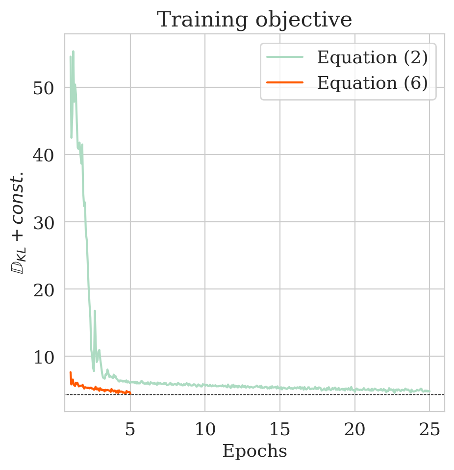
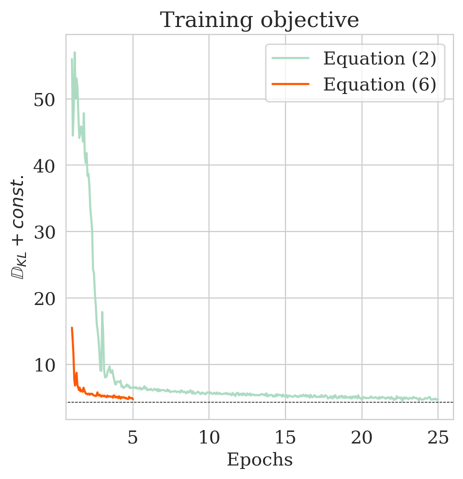
We observe that by decreasing \(\gamma\) from \(2\) to \(0\), the low-fidelity posterior approximations become worse. As a result, the objective function for the preconditioned approach (orange) at the beginning start from a higher value, indicating more mismatch between low- and high-fidelity posterior densities. Finally, our preconditioning method consistently improves upon low-fidelity posterior by training for \(5\) epochs.

Seismic compressed sensing—more results

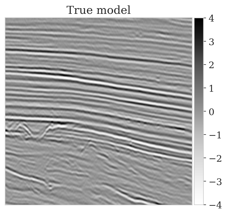
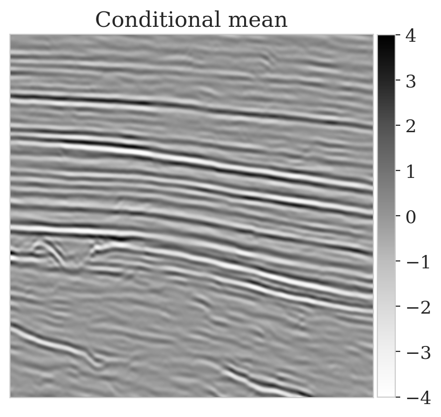
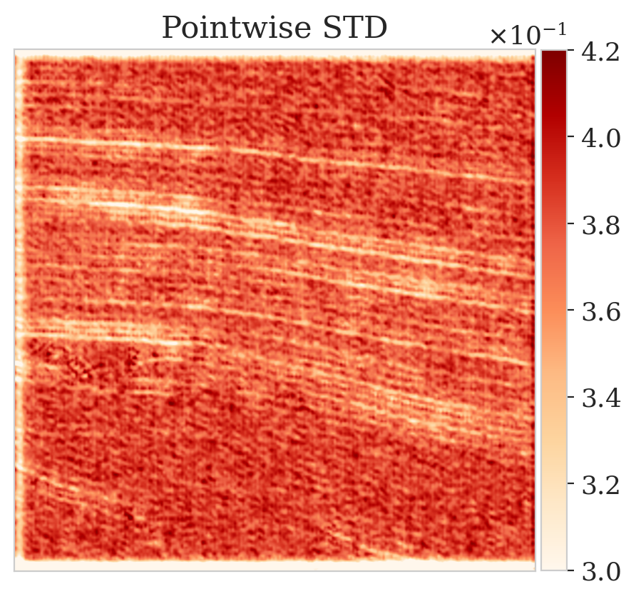
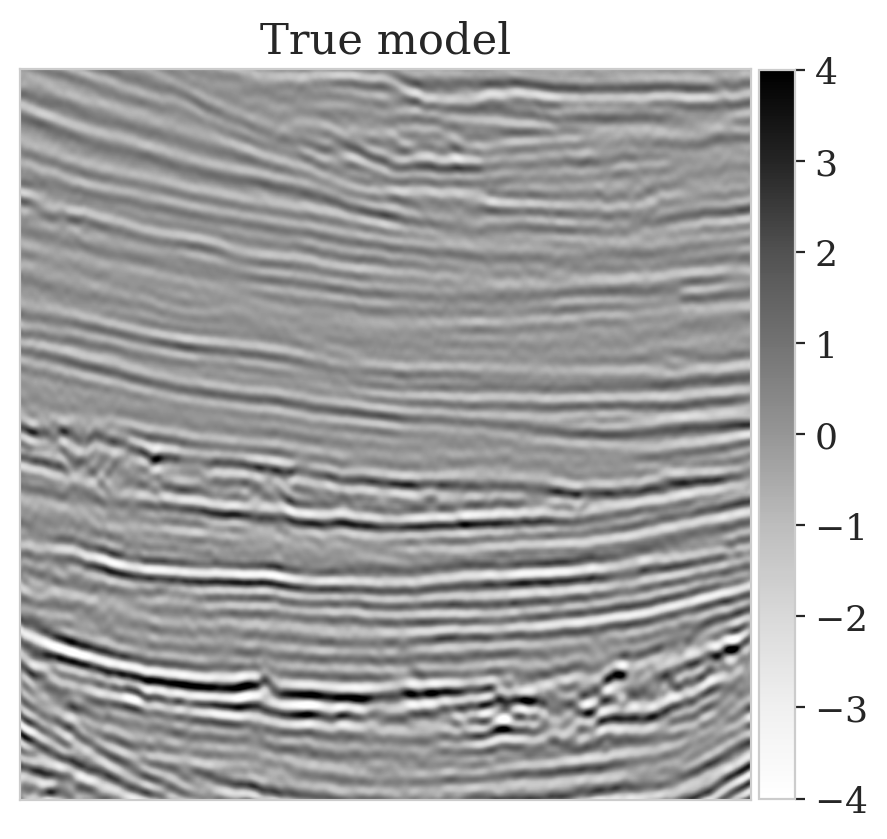
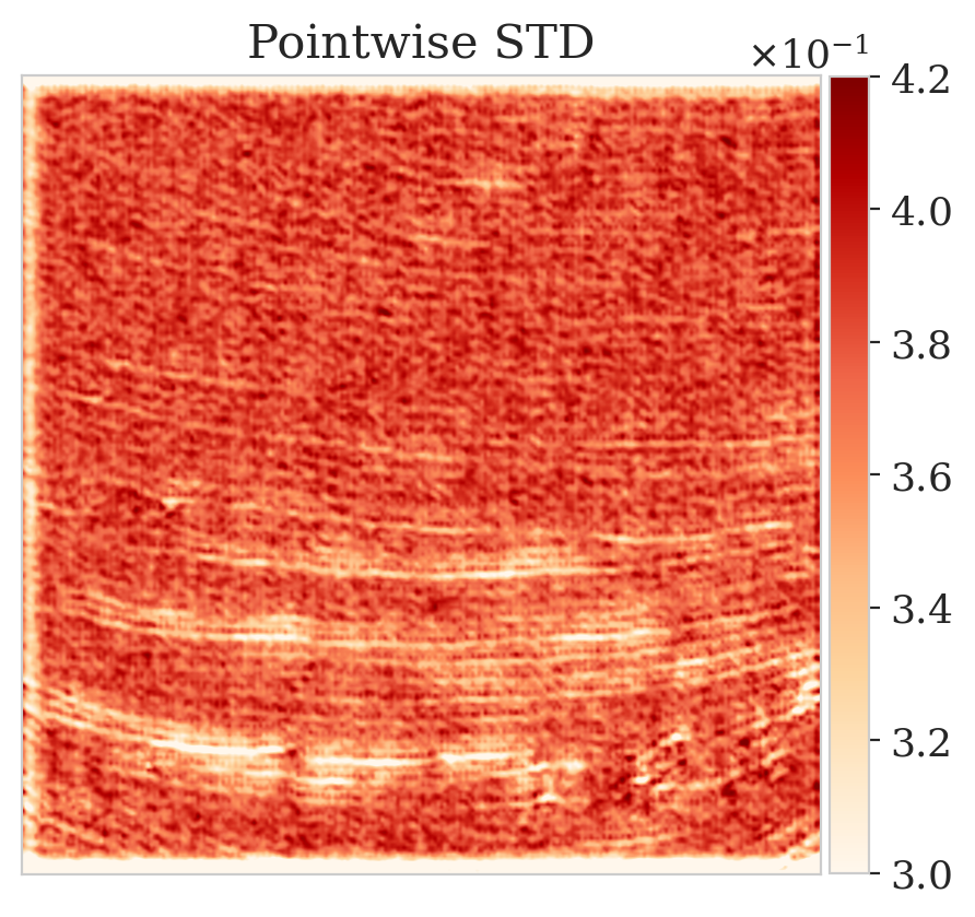
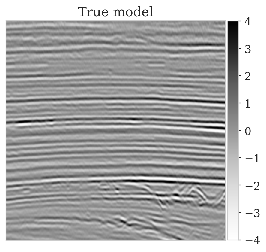
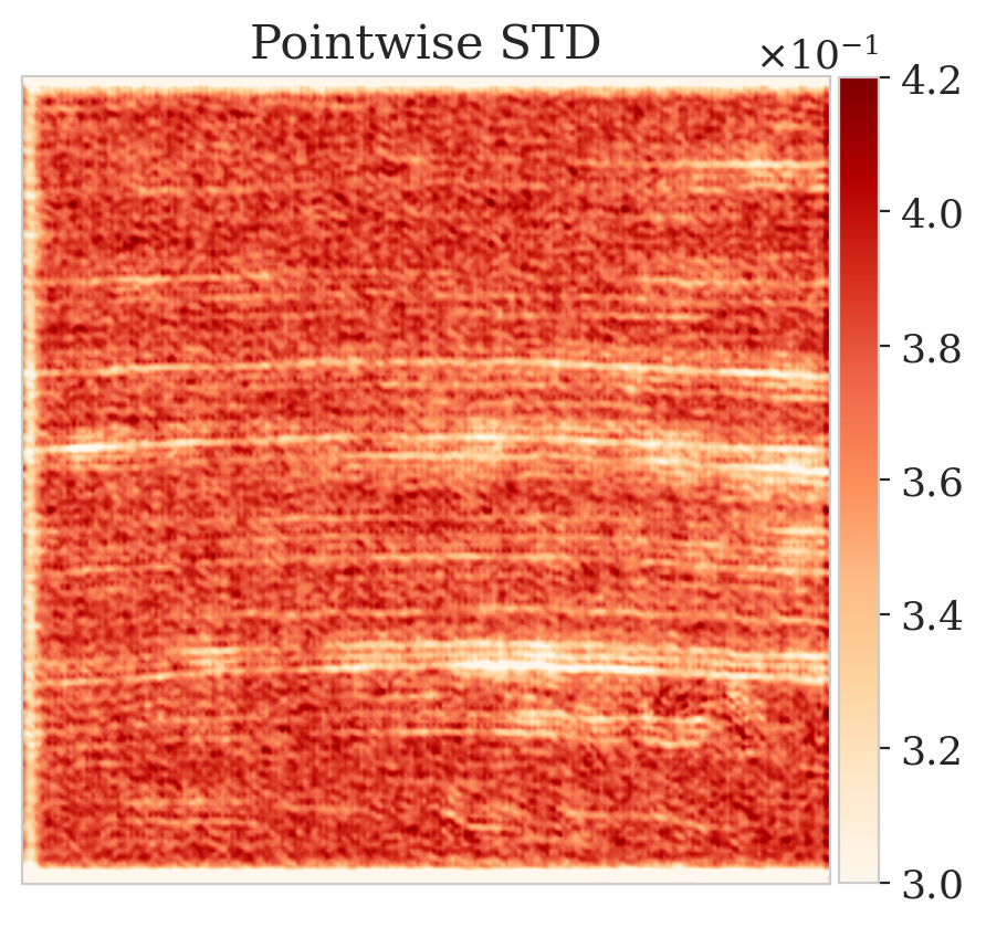
Here we show more examples to verify the pretraining phase obtained via solving the objective in Equation (\(\ref{hint2-obj}\)). Each row in Figure 5 corresponds to a different testing image. The first column shows the different true seismic images used to create low-fidelity compressive sensing data, depicted in the second column. The third and last columns correspond to the conditional mean and pointwise STD estimates, respectively. Clearly, the pretrained network is able to successfully recover the true image, and consistently indicates more uncertainty in areas with low-amplitude events.